University Notes - Computer Science

Just code and projects for university. All the study-related contents are just a summary of the actual material. For better explanations check other material here, study on books suggested by the teachers and learn by writing your own material 😀

You are encouraged to follow the lectures and do exercises over and over again. The process of learning requires effort

A pottery teacher split her class into two halves

To the first half she said, "You will spend the semester studying pottery, planning, designing, and creating your perfect pot. At the end of the semester, there will be a competition to see whose pot is the best".

To the other half she said, "You will spend your semester making lots of pots. Your grade will be based on the number of completed pots you finish. At the end of the semester, you'll also have the opportunity to enter your best pot into a competition."

The first half of the class threw themselves into their research, planning, and design. Then they set about creating their one, perfect pot for the competition.

The second half of the class immediately grabbed fistfulls of clay and started churning out pots. They made big ones, small ones, simple ones, and intricate ones. Their muscles ached for weeks as they gained the strength needed to throw so many pots.

At the end of class, both halves were invited to enter their most perfect pot into the competition. Once the votes were counted, all of the best pots came from the students that were tasked with quantity. The practice they gained made them significantly better potters than the planners on a quest for a single, perfect pot.

Original Post

Un'occhiata veloce a GitHub Classroom

Sarò molto sintetico, solo per dare un'idea di come funzionano gli esercizi e il feedback agli studenti

Home

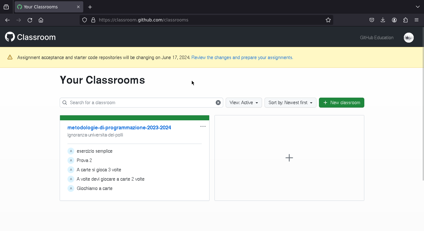
Creare una "Classroom"

Per creare una "Classroom" bisogna selezionare l'organizzazione nella quale si vogliono mettere i repository (si quelli con le soluzioni degli studenti, sia i template con i test)

Una possibile organizzazione per il corso potrebbe essere "Metodologie di programmazione Sapienza"

Passiamo direttamente alle informazioni importanti

Amministratori della "Classroom"

Si può usare un link d'invito per decidere i docenti (amministratori) del corso

Assegnare esercizi

Una volta creata la "Classroom", questa è l'interfaccia di gestione dei degli esercizi

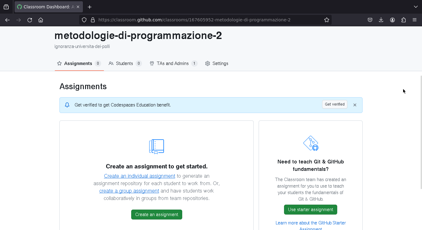
Individuale, di gruppo, pubblico o privato (scadenza opzionale)

Per assegnare un esercizio bisogna dare alcune informazioni di base: il nome, un'eventuale scadenza (opzionale), se si tratta di un esercizio di gruppo o individuale.

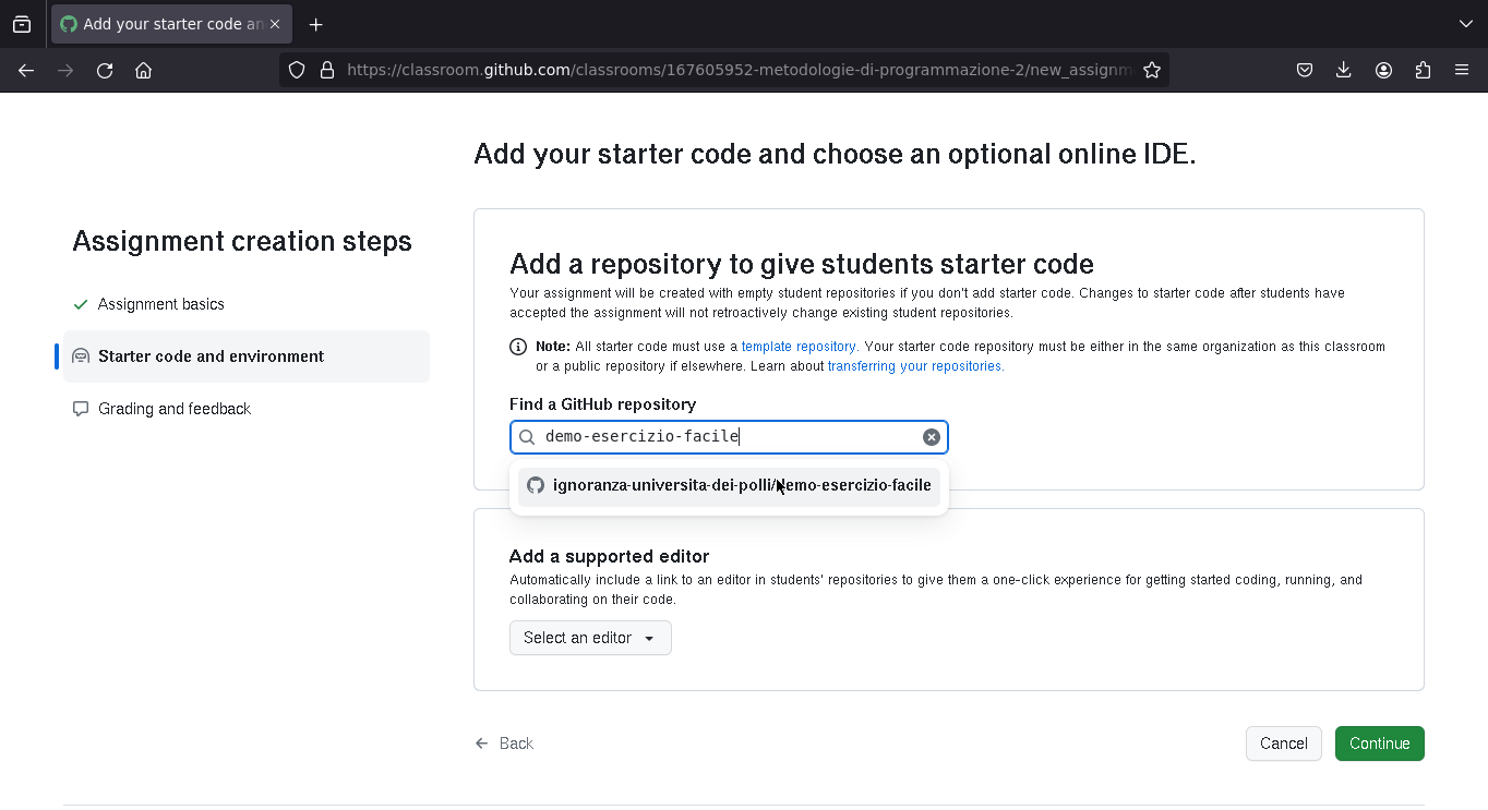
Quando lo studente "accetterà l'esercizio", verrà creato un repository (pubblico o privato) con il nome dell'esercizio e dello studente nell'organizzazione che avevamo scelto nella creazione della "Classroom"

Successivamente, si sceglie il template (il repository con i test) da usare per l'esercizio (i template con i test vengono creati una volta, e si riusano ogni anno)

Template da usare per l'esrecizio

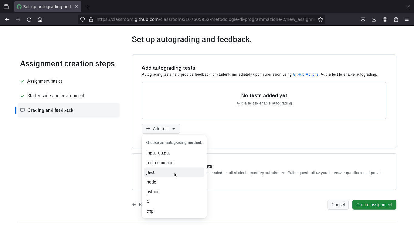
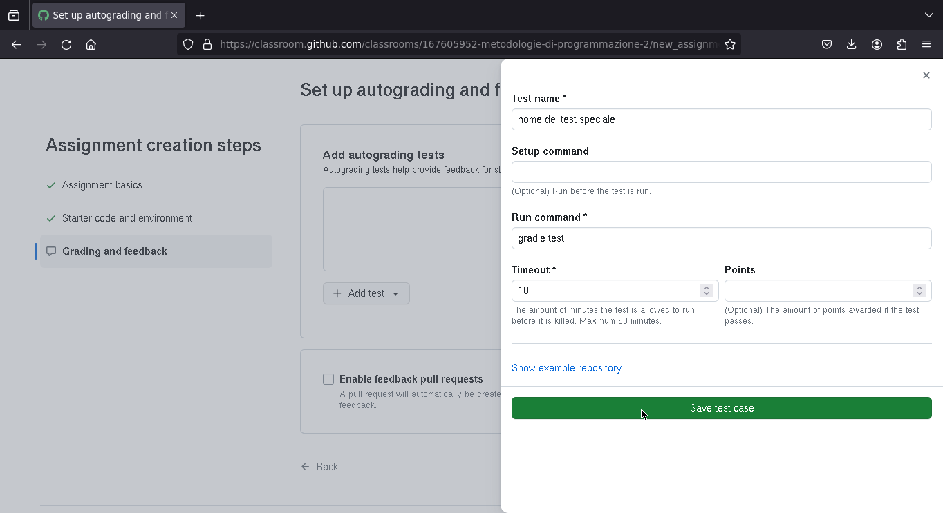
Test

Qui si può decidere di eseguire un comando unico che fa girare tutti i test (quindi l'esercizio può essere passato / non passato), oppure si può decidere di andare più a grana fine e far girare più comandi che eseguono ciascuno un sottoinsieme dei test.

Riusare i test per gli anni futuri

Gli esercizi si possono riusare, quindi non è necessario ogni volta riscrivere i test per gli esercizi dell'anno passato. Si può prendere un esercizio dell'anno passato, cliccare il tasto "riusa" e si può riproporre lo stesso esercizio con gli stessi test in un anno successivo.

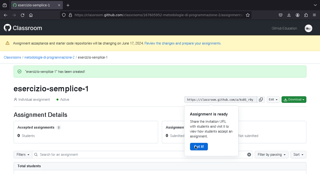
Condivisione esercizio

Una volta creato l'esercizio viene generato un link. Se gli studenti cliccano su quel link, possono accettare di fare l'esercizio, caso in cui viene creato un repository per il studente.

Svolgere gli esercizi

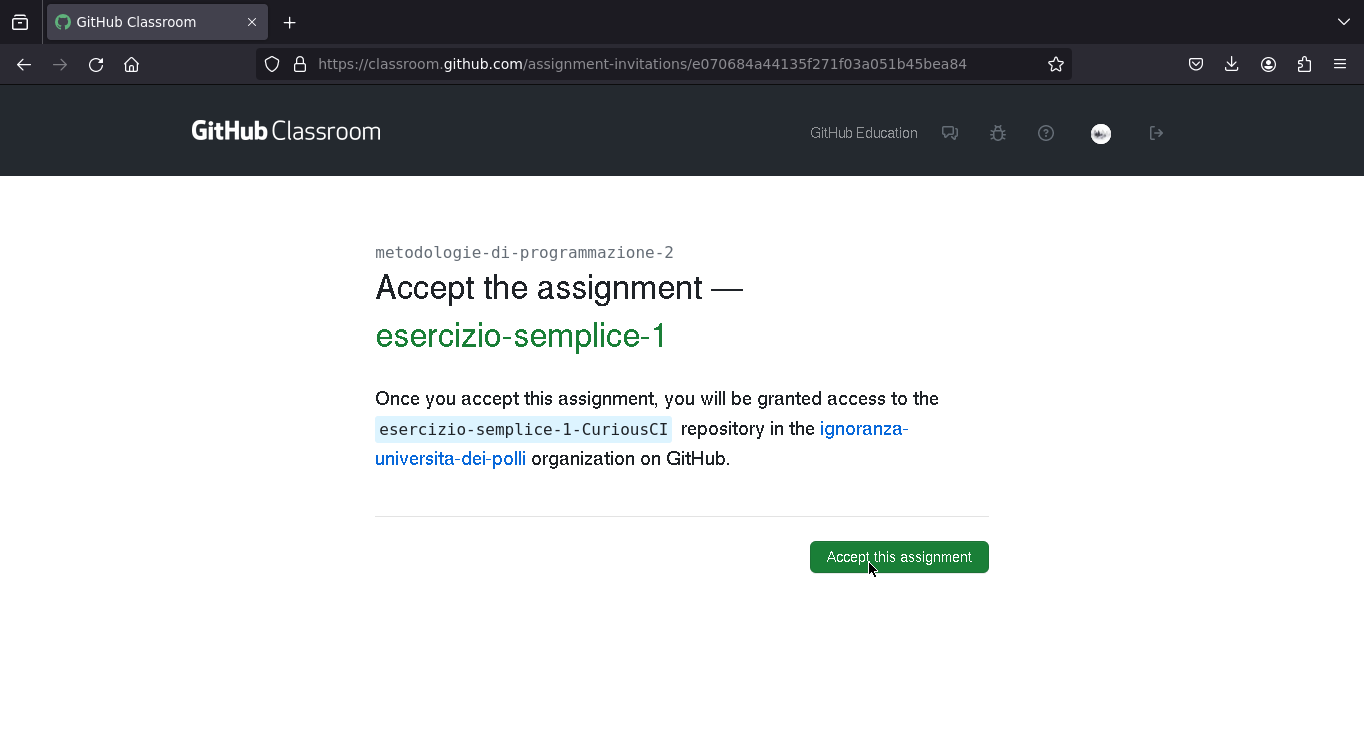
Accettare un homework

Questa è la schermata che vede uno studente quanto clicca un esercizio (se volete provare questo è il link di un esercizio https://classroom.github.com/a/lWBDk-we)

Link del repository appena creato

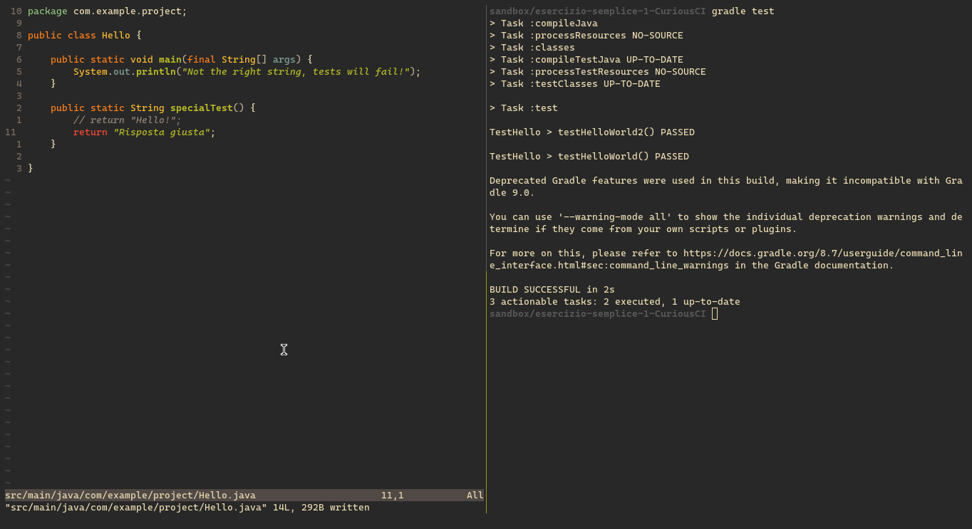
Testare in locale

Lo studente dovrà clonare il repository in locale (lo si può fare da CLI come preferisco io, altrimenti Eclipse ha integrate le funzionalità per lavorare con git e GitHub)

In questo esempio, per far girare i test ho eseguito il comando gradle test, per chi usa Eclipse, è già tutto integrato nell'editor, e possono eseguire i test cliccando sul tasto verder per eseguire il programma.

Qui un test fallisce.

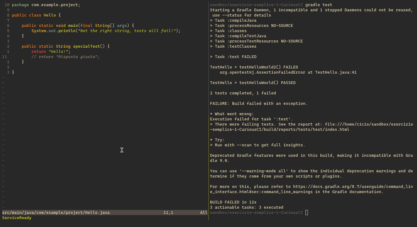
Lo studente scrive il codice per far funzionare il test. Ora i 2 test passano enrambi.

Pubblicare il codice

Una volta risolto l'esercizio (o anche parte di esso!) lo studente può fare il commit del codice al repository generato prima (usando git da CLI come nel mio caso, altrimenti Eclipse ha integrate le funzionalità per farlo in modo semplice)

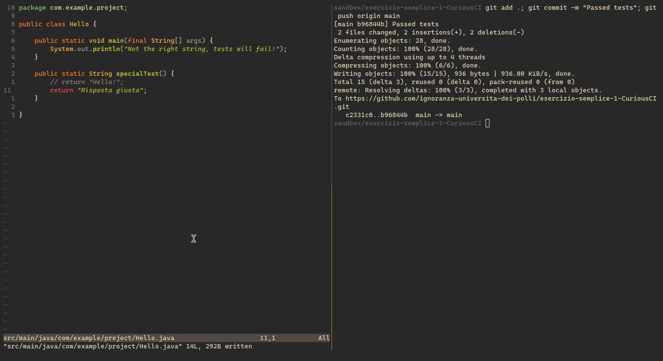
GitHub testa in automatico il codice

Quando lo studente fa il commit del codice, GitHub si occupa anche lui di esegure i test, per far vedere al docente quanti e quali test ha superato fino a quel momento lo studente.

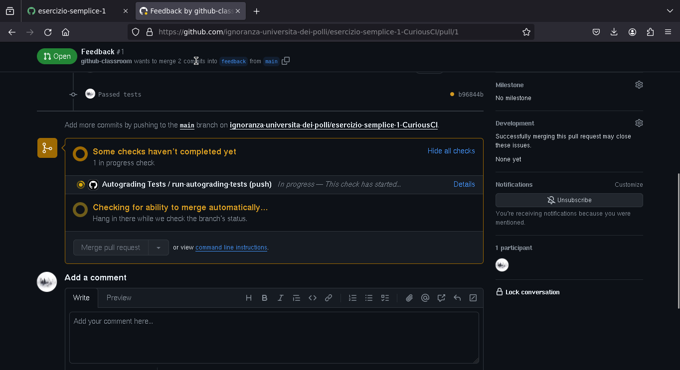
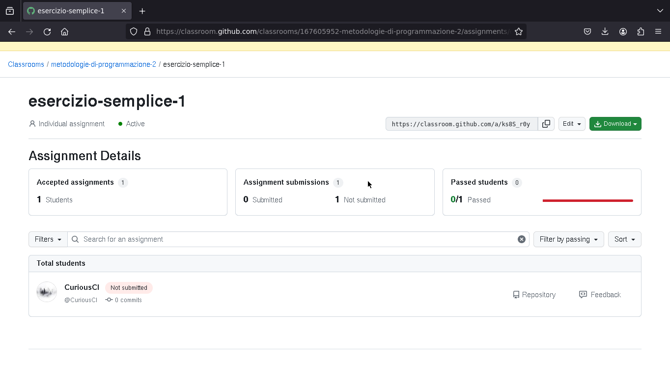
Esercizi dal punto di vista del doecente

Il docente può vedere l'elenco degli studenti che hanno accettato di fare l'esercizio, se hanno passato o meno i test, e possono andare a vedere il codice che hanno scritto (e lasciare un eventuale feedback manuale sul codice)

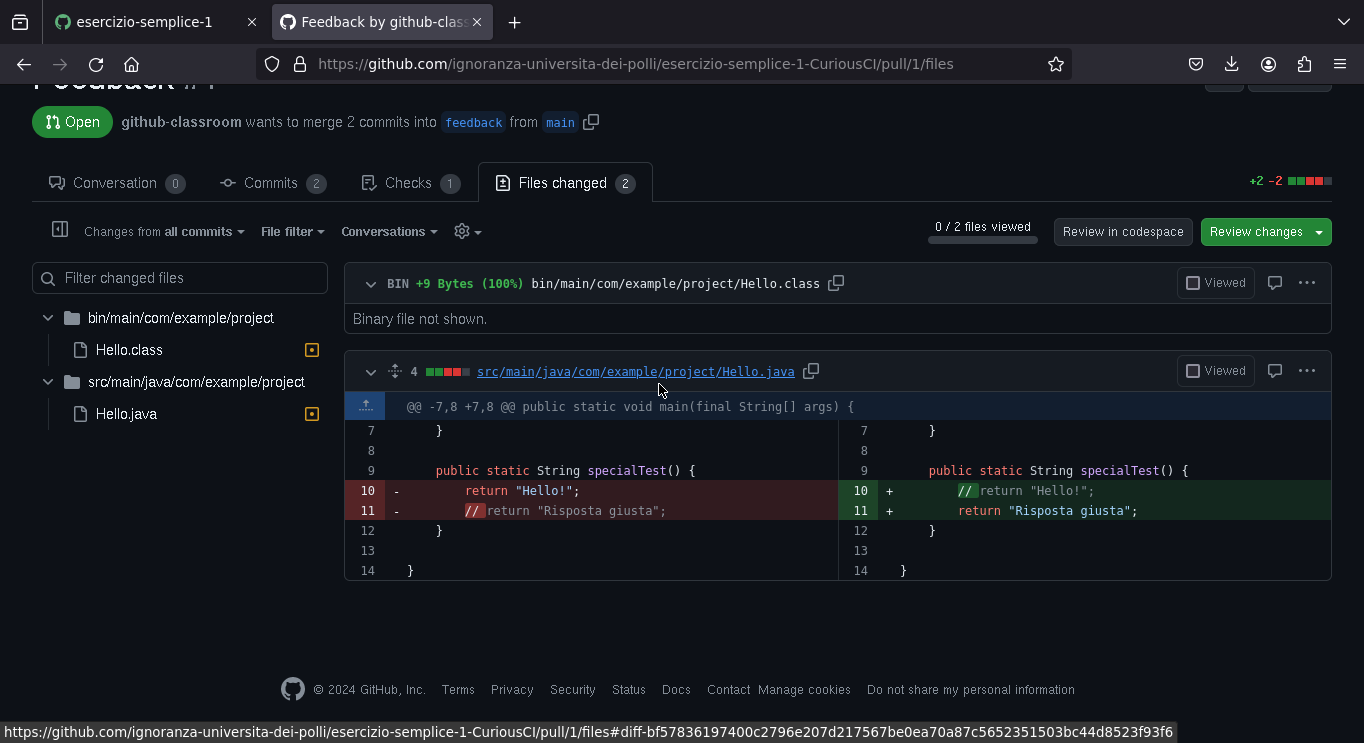
Feedback del docente

Eventualmente, il docente può vedere il codice che ha scritto lo studente.

Computer Architecture

1951 IAS Machine Architecture

This section is made to grasp a basic understand of how a computer architecture works, and it's not meant to be studied thoroughly.

The IAS Machine had a 1000 word memory, with a 40b word (40000b = 5000B ~ 5kB).

Word

Words are CA2 integers

Instruction words contain two instructions

CPU

Instructions

This isn't the full ISA of the IAS Machine, check it out here.

Transfer Instructions

Jumps

Like in modern assembly, jumps can be unconditional, conditional; for the IAS machine you had to specify either a low or high address.

Operations

Example Program

LOAD 101
ADD 102
ST 103

How does it work?

1. Fetch
   • MAR \(\leftarrow\) PC
   • IR, IBR \(\leftarrow\) MBR \(\leftarrow\) Memory[MAR]
2. Decode
   • MAR \(\leftarrow\) IR[8..19] ; address
   • CU \(\leftarrow\) IR[0..8] ; opcode
3. Exec
   • AC \(\leftarrow\) MBR \(\leftarrow\) Memory[101]
4. Decode
   • MAR \(\leftarrow\) IBR[8..19] ; address
   • CU \(\leftarrow\) IBR[0..8] ; opcode
5. Exec
   • AC \(\leftarrow\) AC + MBR \(\leftarrow\) Memory[102]
6. PC
   • PC \(\leftarrow\) PC + 1
7. Fetch
   • MAR \(\leftarrow\) PC
   • IR, IBR \(\leftarrow\) MBR \(\leftarrow\) Memory[MAR]
8. Decode
   • MAR \(\leftarrow\) IR[8..19] ; address
   • CU \(\leftarrow\) IR[0..8] ; opcode
9. Exec
   • Memory[103] \(\leftarrow\) MBR \(\leftarrow\) AC

MIPS

RISC vs CISC

Reduced Instruction Set Computer vs Complex Instruction Set Computer

Registers

Special registers

• $gp\ast \ast pointsintothemiddleofa\ast \ast 64Kblock\ast \ast ofmemoryinthe\ast \ast heap\ast \ast thatholdsconstantsand\ast \ast globalvariables\ast \ast -\ast \ast$sp points to the last location in use on the stack
• $fp\ast \ast pointstothestartofthestackframeanddoesnotmoveforthedurationofthesubroutinecall,andtheparametersthatarepassedintothesubroutineremainataconstantspotrelativetotheframepointer-\ast \ast$ra is written with the return address for a call by the jal instruction

Instructions

R-type Instructions

Arithmetic Instruction Format (type to a register)

add $t0, $s1, $s2

• add opcode \(\to\) 000000
• $$\begin{gathered} t0in\ast \ast rd\ast \ast \\ (\to \\ )01000- \end{gathered}$$s1 in rs, \(\to\) 10001
• s2 in rt, \(\to\) 10010
• add funct \(\to\) 100000

I-type Instructions

Data Transfer Format (conditional jumps)

addi t2, <span class="katex"><span class="katex-html" aria-hidden="true"><span class="base"><span class="strut" style="height:0.8889em;vertical-align:-0.1944em;"></span><span class="mord mathnormal">s</span><span class="mord">2</span><span class="mpunct">,</span><span class="mspace" style="margin-right:0.1667em;"></span><span class="mord">4‘‘‘</span><span class="mspace" style="margin-right:0.2222em;"></span><span class="mbin">−</span><span class="mspace" style="margin-right:0.2222em;"></span></span><span class="base"><span class="strut" style="height:0.6944em;"></span><span class="mord mathnormal">a</span><span class="mord mathnormal">dd</span><span class="mord mathnormal">i</span><span class="mspace" style="margin-right:0.2222em;"></span><span class="mbin">∗</span><span class="mspace" style="margin-right:0.2222em;"></span></span><span class="base"><span class="strut" style="height:0.8889em;vertical-align:-0.1944em;"></span><span class="mord">∗</span><span class="mord mathnormal">o</span><span class="mord mathnormal">p</span><span class="mord mathnormal">co</span><span class="mord mathnormal">d</span><span class="mord mathnormal">e</span><span class="mspace" style="margin-right:0.2222em;"></span><span class="mbin">∗</span><span class="mspace" style="margin-right:0.2222em;"></span></span><span class="base"><span class="strut" style="height:0.4653em;"></span><span class="mord">∗</span></span><span class="mspace newline"></span><span class="base"><span class="strut" style="height:1em;vertical-align:-0.25em;"></span><span class="mopen">(</span><span class="mrel">→</span></span><span class="mspace newline"></span><span class="base"><span class="strut" style="height:1em;vertical-align:-0.25em;"></span><span class="mclose">)</span><span class="mord">001000</span><span class="mord">−</span></span></span></span>t2 in **rt** \\(\to\\) 01010
- s2 in **rs** \\(\to\\) 10010

| op | rs | rt | constant |
|:--:|:--:|:--:|:--:|
| 001000 | 10010 | 01010 | 0000000000000100 |
| 6b | 5b | 5b | 16b |
| opcode | first <br/> register | target <br/> register | constant value or <br/> address | 

<!-- | \\(0..5\\) | \\(6..10\\) | \\(11..15\\) | \\(16..31\\) | -->

### J-type Instructions

Unconditional Jumps

```armasm
j label

• PC \(\leftarrow\) label \(\cdot\) 4

FR-type Instructions

MIPS handles floating point instructions like regular 32b instructions. FR-type don't access the memory, and are executed by the FPU.

add.s f0, <span class="katex"><span class="katex-html" aria-hidden="true"><span class="base"><span class="strut" style="height:0.8889em;vertical-align:-0.1944em;"></span><span class="mord mathnormal" style="margin-right:0.10764em;">f</span><span class="mord">1</span><span class="mpunct">,</span></span></span></span>f2 ; single precision
div.d <span class="katex"><span class="katex-html" aria-hidden="true"><span class="base"><span class="strut" style="height:0.8889em;vertical-align:-0.1944em;"></span><span class="mord mathnormal" style="margin-right:0.10764em;">f</span><span class="mord">0</span><span class="mpunct">,</span></span></span></span>f2, f4 ; double precision

FI-type Instructions

FI-type are used for:

• load / store
• conditional jumps

lwc1 f1, indirizzo
bc1f cc, offset

Interrupts

TODO: Interrupts

Assembly

wiki

Compilation

TODO: fill this section with instructions on how to compile assembly code

• .s -> .o

• .o -> .exe linking

• windows

• linux

Memory Layout of a Program

Directives

.globl

The .globl directive is useful when working with multiple files, and we need parts of code to reference labels in other files. If you don't use .globl, during the linking process, it can't find the label and gives an error.

We could have a main.asm file like this:

.globl main
.data
.text
    main: 
        li $a0, 5
        jal fibonacci
        ...

And a second file math.asm with the fibonacci function:

.globl fibonacci
.data
.text
    fibonacci:
       mv $t0, $a0 
       ...

.ent

There is a .ent directive too, which is a debugger pseudo operation that marks the entry of main.

.globl main
.ent main
.text
    main:
        ...

Pseudo-Instructions

Many instructions provided by MIPS, like move, lw etc... are decomposed into multiple instructions when the code is assembled; for more details. For example:

lw

lw $s0, value is mapped to:

lui $1, 0x00001001
lw $16, 0x00000000($1)

In the second case, 0x10010000 is the address of value, to get this address, we need to lui 0x00001001 (load upper immediate, loads the immediate value in the upper 16bits of the $1 register, which is the $at register). Then we can load into $16, which is the $s0 register, whatever value is at the address 0 + $at (0x00000000($1))

move

move $t0, $s0 is mapped to addu $8, $0, $16, where addu is the "add unsigned" operation, and $8 is $t0, $0 is the $zero constant register and $16 the $s0 register.

beq

ble $s1, $t0, label is mapped to:

slt $1, $8, $17
beq $1, $0, 0x00000001

Now, slt (set less than) sets the value in rs to 1 if rt is less than rd (if you don't know what rs, rt and rd are, check R-Type Instructions)

Absolute Jump

MIPS instructions have a fixed 32 bit size... what happens when you need to jump to an address which is a 32 bit constant? Neither I-type or J-type support 32 bit constants. We need to use lui and ori.

Let's suppose we have to jump at the address 0000_0000_1111_1111_0000_1001_0000_0000, which corresponds to 0x00ff0900.

lui $t0, 0x000000ff
ori $t0, 0x00000900
jr $t0

What lui does is moving the lower 16 bits 0x00ff into the upper part of register $t0, that way we have 0x00ff0000 in $t0. Now, we use ori (which does a bitwise or, basically compares with an or for each bit in $t0 with the value 0x00000900 for the lower half of the byte) so we have the full address. Now we can just use jr to jump to the address in the register.

Statements

For each statement, I'll show the C code (I chose C over other languages as the generated assembly is very minimal and easy to understand), and the relative MIPS implementation; under details I'll leave the x_86 assembly generated by cl.exe on Windows and gcc on Linux.

Conditions

If-Else

int main() {
  int x = 0;

  if (x > 0)
    x += 5;
  else
    x += 10;
}

.text
    li $t0, 0 #; x = 0

    blez $t0, else #; if x <= 0, goto else

    if:
        addi $t0, $t0, 5 #; add 5 to x if x > 0
        j end #; don't execute else part
    else: 
        addi $t0, $s1, 10 #; add 10 to x if x <= 0
    end:

Switch

int main() {
  int x = 1;

  switch (x) {
  case 0:
    x += 16;
    break;
  case 1:
    x += 16 * 2;
    break;
  case 2:
    x += 16 * 3;
    break;
  }
}

.data
    dest: .word case0, case1, case2
.text
    #; sll $t0, $t0, 2 #; choose the case

    li $t0, 0 #; first case 
    addi $t0, $t0, 4 #; jump one case
    #; addi $t0, $t0, 8 #; jump two cases

    lw $t1, dest($t0) #; load case address to $t1
    jr $t1 #; Jump to the case address in $t1 (case0, case1 etc...)

    li $t2, 0
    case0:
        addi $t2, $zero, 0x10
        j break 
    case1:
        addi $t2, $zero, 0x20
        j break 
    case2:
        addi $t2, $zero, 0x30
        j break 
    break:

Iterations

Do-While

int main() {
  int x = 0, i = 0;

  do {
    x += 4;
    i += 1;
  } while (i < 10);
}

.text
    li $t0, 0 #; x = 0
    li $t1, 0 #; i = 0

    do:
        addi $t0, $t0, 4 #; x += 4
        addi $t1, $t1, 1 #; i += 1
    blt $t1, 10, do #; if i < 10, repeat the cicle 

While

int main() {
  int x = 0, i = 0;

  while (i < 10) {
    x += 4;
    i += 1;
  }
}

.text
    li $t0, 0 #; x = 0
    li $t1, 0 #; i = 0

    while:
        bge $t1, 10, end #; if i >= 10, end the while loop
        addi $t0, $t0, 4 #; x += 4
        addi $t1, $t1, 1 #; i += 1
        j while #; repeat cicle
    end:

For

int main() {
  int x = 0;

  for (int i = 0; i <= 10; i++)
    x += i;
}

.text
    li $t0, 0 #; x = 0
    li $t1, 0 #; i = 0

    for:
        beq $t1, 10, end #; if i == 10, end loop 
        add $t0, $t0, $t1 #; x += i
        addi $t1, $t1, 1 #; i += 1 
        j for
    end:

Vectors & Matrices

Endianness

The MIPS architecture allows both big-endian and little-endian byte ordering, but the little-endian one is most commonly used. Endianness has to do on how bytes are addressed in memory, and it's related to how the access of each individual byte is made.

ASCII

TODO ASCII

Vectors

There are many types of vectors you can handle in MIPS:

.data
    byte: .byte 29, 8, 1, 29, 2, -3
    half: .half 10, -4, 20, -8, 22, 12
    word: .word 2, 29012, 29, 5, -12905, -290125

    # decimal 

    float: .float 2.5, -1.2, 21.90, -5.0
    double: .double 2.5, -1.2, 21.90, -5.0

    # strings

    string: .asciiz "Holy Moly, who ate my Canoli?"

Note that .asciiz stands for "zero terminated string", which means it has a '\0' nullchar at the end.

Vector Iterations

You can iterate vectors and matrices in two ways:

Index

• useful if you need the index of each element
• the increment of the index doesn't depend on the size of the elements
• you have to convert the index each time, according to the size of the elements

.data
    vector: .word 10, 2, 980, 29, 1992, -2, 59, 280, 99
    size: .word 9
.text
    la $s0, vector #; s0 = vector address
    la $t1, size #; t1 = address of size
    lw $t1, ($t1) #; t1 = size

    li $t0, 0 #; t0 is the index i

    for:
        bge $t0, $t1, end #; if i == size, end loop

        sll $t2, $t0, 2 #; offset = i * 4 (shift logic left by 2)
        addi $t2, $t2, $s0 #; t2 = current address = offset + address

        lw $t7, ($t2) #; load value from current address, and maybe use it

        #; rest of the code ...

        addi $t0, $t0, 1 #; i = i + 1
        j for #; loop again
    end:

TODO: check if it works

Pointer

• you work directly with the address
• less calculations to do in the cycle
• you don't have the index of the element
• the increment depends on the size of the elements
• you must calculate the index after the last element

.data
    vector: .word 10, 2, 980, 29, 1992, -2, 59, 280, 99
    size: .word 9
.text
    la $t0, vector #; t0 = vector address

    la $t1, size #; t1 = address of size
    lw $t1, ($t1) #; t1 = size
    sll $t1, $t1, 2 #; size = size * 4 (we are handling words)
    add $t1, $t0, $t1 #; t1 = end address = vector address + size * 4 (this is the address after the last one in the vector)

    for:
        bge $t0, $t1, end #; if current address == vector end address, end loop

        lw $t7, ($t0) #; load value from current address, and maybe use it

        #; rest of the code ...

        addi $t0, $t0, 4 #; current address = current address + 4 (we move by 4 bytes, because we are using words) 
        j for #; loop again
    end:

TODO: check if it works

Matrices

If you want a 7 (rows) x 13 (columns) matrix, you need enough space for 91 elements:

.data
    matrix: .word 0:91

Matrixes are stored in memory like vectors, each row is laid one after the other. To work with n-sized matrices, you just lay out one matrix after the other in memory (you can have a 3-dimensional matrix, for example, where the z coordinate dictates the layer, or the matrix, you are working with)

Syscalls & Procedures

Syscalls

Syscalls are a powerful tool, which enables interaction with I/O, files, and dynamic allocation of memory. The MARS editor supports 59 different syscalls. Here's a few of useful ones.

To use syscalls, there are some special registers:

• $v0 is used for the code of the syscall
• $a0 to $a3 are used for parameters
• The output is usually saved in $v0

By setting these registers to the desired values, and using the syscall instruction, the OS will run the operation.

| service | $v0|arguments|output||--|--|--|--||printinteger|1|$a0 = integer to print | | | print string | 4 | $a0=addressofnull-terminatedstringtoprint|||readinteger|5||$v0 contains integer read | | | read string | 8 | $a0=addressofinputbuffer<br/>$a1 = maximum number of characters to read | | | sbrk (allocate heap memory) | 9 | $a0=numberofbytestoallocate|$v0 contains address of allocated memory | | print character | 11 | $a0=charactertoprint|||readcharacter|12||$v0 contains character read | | exit | 10 | | | | exit2 | 17 | a0 = result | |

Files

Hello World!

.globl main

.data
    string: .asciiz "Hello World!"

.text
    main: 
        li v0, 4
        la a0, string
        syscall

Procedures

Procedures are pieces of code that take parameters, and return a result. They're useful to make the code cleaner and more modular.

.globl main

.text
    main:
        li a0, 5 #; first parameter
        li a1, 6 #; second parameter
        jal function #; call function

        return:
            li v0, 17
            li a0, 0
            syscall #; we have to exit, or the execution will continue

    function:
        subi sp, sp, 12 #; we need 4 bytes * 3 registers 
        sw ra, 8(sp) #; return address
        sw a0, 4(<span class="katex"><span class="katex-html" aria-hidden="true"><span class="base"><span class="strut" style="height:1em;vertical-align:-0.25em;"></span><span class="mord mathnormal">s</span><span class="mord mathnormal">p</span><span class="mclose">)</span><span class="mord mathnormal">s</span><span class="mord mathnormal" style="margin-right:0.02691em;">w</span></span></span></span>a1, 0(sp)

        #; function body...
        #; I can use jal, because we have saved in memory ra

        lw <span class="katex"><span class="katex-html" aria-hidden="true"><span class="base"><span class="strut" style="height:1em;vertical-align:-0.25em;"></span><span class="mord mathnormal">a</span><span class="mord">1</span><span class="mpunct">,</span><span class="mspace" style="margin-right:0.1667em;"></span><span class="mopen">(</span></span></span></span>sp)
        lw <span class="katex"><span class="katex-html" aria-hidden="true"><span class="base"><span class="strut" style="height:1em;vertical-align:-0.25em;"></span><span class="mord mathnormal">a</span><span class="mord">0</span><span class="mpunct">,</span><span class="mspace" style="margin-right:0.1667em;"></span><span class="mord">4</span><span class="mopen">(</span></span></span></span>sp)
        lw <span class="katex"><span class="katex-html" aria-hidden="true"><span class="base"><span class="strut" style="height:1em;vertical-align:-0.25em;"></span><span class="mord mathnormal" style="margin-right:0.02778em;">r</span><span class="mord mathnormal">a</span><span class="mpunct">,</span><span class="mspace" style="margin-right:0.1667em;"></span><span class="mord">8</span><span class="mopen">(</span></span></span></span>sp)
        addi <span class="katex"><span class="katex-html" aria-hidden="true"><span class="base"><span class="strut" style="height:0.625em;vertical-align:-0.1944em;"></span><span class="mord mathnormal">s</span><span class="mord mathnormal">p</span><span class="mpunct">,</span></span></span></span>sp, 12 #; reset stack pointer
        
        jr <span class="katex"><span class="katex-html" aria-hidden="true"><span class="base"><span class="strut" style="height:0.8889em;vertical-align:-0.1944em;"></span><span class="mord mathnormal" style="margin-right:0.02778em;">r</span><span class="mord mathnormal">a</span><span class="mord">‘‘‘</span><span class="mord mathnormal" style="margin-right:0.13889em;">T</span><span class="mord mathnormal">h</span><span class="mord mathnormal">e</span><span class="mord mathnormal">b</span><span class="mord mathnormal" style="margin-right:0.01968em;">l</span><span class="mord mathnormal">oc</span><span class="mord mathnormal" style="margin-right:0.03148em;">k</span><span class="mord mathnormal">t</span><span class="mord mathnormal">h</span><span class="mord mathnormal">e</span><span class="mord mathnormal" style="margin-right:0.10764em;">f</span><span class="mord mathnormal">u</span><span class="mord mathnormal">n</span><span class="mord mathnormal">c</span><span class="mord mathnormal">t</span><span class="mord mathnormal">i</span><span class="mord mathnormal">o</span><span class="mord mathnormal">n</span><span class="mord mathnormal">t</span><span class="mord mathnormal" style="margin-right:0.03148em;">ak</span><span class="mord mathnormal">es</span><span class="mord mathnormal" style="margin-right:0.10764em;">f</span><span class="mord mathnormal">ro</span><span class="mord mathnormal">m</span><span class="mord mathnormal">t</span><span class="mord mathnormal">h</span><span class="mord mathnormal">e</span><span class="mspace" style="margin-right:0.2222em;"></span><span class="mbin">∗</span><span class="mspace" style="margin-right:0.2222em;"></span></span><span class="base"><span class="strut" style="height:0.6944em;"></span><span class="mord">∗</span><span class="mord mathnormal">s</span><span class="mord mathnormal">t</span><span class="mord mathnormal">a</span><span class="mord mathnormal">c</span><span class="mord mathnormal" style="margin-right:0.03148em;">k</span><span class="mspace" style="margin-right:0.2222em;"></span><span class="mbin">∗</span><span class="mspace" style="margin-right:0.2222em;"></span></span><span class="base"><span class="strut" style="height:0.6944em;"></span><span class="mord">∗</span><span class="mord mathnormal">i</span><span class="mord mathnormal">sc</span><span class="mord mathnormal">a</span><span class="mord mathnormal" style="margin-right:0.01968em;">ll</span><span class="mord mathnormal">e</span><span class="mord mathnormal">d</span><span class="mspace" style="margin-right:0.2222em;"></span><span class="mbin">∗</span><span class="mspace" style="margin-right:0.2222em;"></span></span><span class="base"><span class="strut" style="height:0.8889em;vertical-align:-0.1944em;"></span><span class="mord">∗</span><span class="mord mathnormal">s</span><span class="mord mathnormal">t</span><span class="mord mathnormal">a</span><span class="mord mathnormal">c</span><span class="mord mathnormal" style="margin-right:0.03148em;">k</span><span class="mord mathnormal" style="margin-right:0.10764em;">f</span><span class="mord mathnormal" style="margin-right:0.02778em;">r</span><span class="mord mathnormal">am</span><span class="mord mathnormal">e</span><span class="mspace" style="margin-right:0.2222em;"></span><span class="mbin">∗</span><span class="mspace" style="margin-right:0.2222em;"></span></span><span class="base"><span class="strut" style="height:0.4653em;"></span><span class="mord">∗</span><span class="mord mathnormal" style="margin-right:0.02778em;">or</span><span class="mspace" style="margin-right:0.2222em;"></span><span class="mbin">∗</span><span class="mspace" style="margin-right:0.2222em;"></span></span><span class="base"><span class="strut" style="height:0.6944em;"></span><span class="mord">∗</span><span class="mord mathnormal">a</span><span class="mord mathnormal">c</span><span class="mord mathnormal">t</span><span class="mord mathnormal">i</span><span class="mord mathnormal" style="margin-right:0.03588em;">v</span><span class="mord mathnormal">a</span><span class="mord mathnormal">t</span><span class="mord mathnormal">i</span><span class="mord mathnormal">o</span><span class="mord mathnormal">n</span><span class="mord mathnormal" style="margin-right:0.02778em;">recor</span><span class="mord mathnormal">d</span><span class="mspace" style="margin-right:0.2222em;"></span><span class="mbin">∗</span><span class="mspace" style="margin-right:0.2222em;"></span></span><span class="base"><span class="strut" style="height:0.6944em;"></span><span class="mord">∗</span><span class="mord">.</span><span class="mord mathnormal" style="margin-right:0.13889em;">W</span><span class="mord mathnormal">ec</span><span class="mord mathnormal">an</span><span class="mord mathnormal">u</span><span class="mord mathnormal">se</span><span class="mord">‘</span></span></span></span>fp` to point to the start of the **activation record**, it's rendundant and rarely used.

## Recursions

Functions calling themselves!

> TODO: complete factorial

```armasm
.globl main

.text
    main:
        li $a0, 5
        jal factorial

        print:
            move $a0, $v0 #; integer = result of factorial function
            li $v0, 1 #; print integer
            syscall

        return:
            li $v0, 17
            li $a0, 0
            syscall

    factorial:
        #; jump by 1
        #; recursive step
        #; base case
        returnFactorial:
            lw $ra, ($sp)
            addi $sp, $sp
            jr $ra

Exercises

These are the implementations of the exercises presentend in course's slides and notations.

; pdf 3 slide 10

.data

.text
    li $s0, 2 #; a = 2
    li $s1, 5 #; b = 5
    li $s2, 9 #; c = 9
    li $s3, 4 #; d = 4
    li $s4, 12 #; e = 12
    
    #; a = ( b - c ) + ( d - e )

    sub $t0, $s1, $s2 #; t0 = b - c
    sub $t1, $s3, $s4 #; t1 = d - e
    add $s0, $t0, $t1 #; s0 = t0 + t1

; pdf 3 slide 11

.data
    variable: 10
    vector: .word 12, 4, 59, 9, 19, 8, 6, 18, 9, 19, 28, 12, 100

.text
    la $s6, variable #; s6 = address of variable
    la $s5, vector #; s5 = address of vector

    #; vector[12] = vector[6] + variable

    lw $t0, ($s6) #; t0 = *s6 (value at address s6, which is the value of the variable)
    lw $t1, 24($s5) #; t1 = s5[6] ; s5[6] = *(s5 + 6), but 6 rappresents words, not bytes, so 6 * 4 = 24 (which corresponds to vector[6])

    add $t0, $t0, $t1 #; t0 += t1 (which is vector[5])

    sw $t0, 48($s5) #; stores result of sum (from t0) to vector[12], but 12 is words, so 48 is bytes

; pdf 3 slide 17

.data

.text
    li $s0, 1 #; u = 1
    li $s1, 0 #; v = 0

    #; v = u * 256

    sll $s1, $s0, 8 #; s1 = s0 * 256

    #; which is the first value that breaks?

    #; a word ha 32 bits, multiplying by 256 means shifting by 8 bits
    #; this means that as soon as we have the 25 bit set to 1, the 1 is shifted out of 32
    #; 2^24 = 16777216

    li $s2, 16777216 #; 16777215 will work normally
    sll $s0, $s2, 8 #; becomes 0

; pdf 4 slide 34

.data 
    vector: .word 11, 35, 2, 7, 29, 95
    size: .word 6

.text
    #; find max value in vector

    la $t0, vector #; t0 = current address
    la $t1, vector #; t1 = end of vector

    la $t2, size #; t2 = address of vector size
    lw $t2, ($t2) #; t2 = vector size
    sll, $t2, $t2, 2 #; t2 *= 4, to accomodate words

    add $t1, $t1, $t2 #; t1 = end of vector + vector size

    lw $t2, ($t0) #; t2 = max value

    for:
        bgt $t0, $t1, endFor #; if current address > end of vector, end for 

        lw $t3, ($t0) #; load value from current address
        ble $t3, $t2, elseSmaller #; if current value <= max value, continue

        ifBigger:
            move $t2, $t3 #; max value = current value

        elseSmaller:

        addi $t0, $t0, 4 #; current address = next address
        j for #; repeat cycle

    endFor:

; pdf 4 slide 35

.data 
    vector: .word 4, -1, 5, 500, 0, 10000, -256
    size: .word 5
    sums: .word 0, 0

.text
    #; find max value in vector

    la $t0, vector #; t0 = current address
    la $t1, vector #; t1 = end of vector

    la $t2, size #; t2 = address of vector size
    lw $t2, ($t2) #; t2 = vector size
    sll, $t2, $t2, 2 #; t2 *= 4, to accomodate words

    add $t1, $t1, $t2 #; t1 = end of vector + vector size

    li $t2, 0 #; t2 = parity 
    li $t4, 0 #; t4 = even 
    li $t5, 0 #; t5 = odd 

    for:
        bgt $t0, $t1, endFor #; if current address > end of vector, end for 

        lw $t3, ($t0) #; load value from current address
        beq $t2, 1, ifIsOdd #; check if current parity is odd

        ifIsEven:
            add $t4, $t4, $t3 #; even += current value
            li $t2, 1 #; parity = odd
            j nextIteration
        ifIsOdd:
            add $t5, $t5, $t3 #; odd += current value
            li $t2, 0 #; parity = even

        nextIteration:
            addi $t0, $t0, 4 #; current address = next address
            j for #; repeat cycle

    endFor:

    la $t6, sums #; t6 = address of the result
    sw $t4, ($t6) #; t6[0] = even 
    sw $t5, 4($t6) #; t6[1] = odd; 4 is used instead of 1 because a word is 4 bytes long

; pdf 5 slide 10 

.data
    vector: .byte 1, 2, 3, 4 
.text
    #; the vector corresponds to the word 0x04030201
    #; which basically is 4, 3, 2, 1
    #; as it's rappresented in memory using little-endian

; pdf 6 slide 7 

.globl main

.data
    matrix: .word 2, -10, -10, -10, 2, -10, -10, -10, 2 
    length: .word 3 

.text
    main: 
        la $t0, matrix #; t0: matrix_address = matrix
        la $t1, length #; t1: matrix_length_address = length 
        lw $t1, ($t1) #; t1: matrix_length = *length
        move $t2, $t1 #; t2: jumps_to_do = matrix_length (to count how many jumps are needed to reach the end)

        addi $t1, $t1, 1 #; t1: jump_length = matrix_length += 1 (to jump to next diagonal cell)
        sll $t1, $t1, 2 #; t1: jump_length = jump_length * 4 (because words are 4 bytes long)

        li $t3, 0 #; t3: sum = 0 

        while:
            beq $t2, 0, end #; if jumps_to_do == 0 { end loop }

            lw $t4, ($t0) #; t4: value = *matrix_address
            add $t3, $t3, $t4 #; sum += value

            subi $t2, $t2, 1 #; jumps_to_do -= 1
            add $t0, $t0, $t1 #; matrix_address = matrix_address = jump_length
            j while
        end:

        print: 
            li $v0, 1 #; print integer
            move $a0, $t3 #; integer = sum
            syscall

        return: 
            li $v0, 17 #; exit
            li $a0, 0 #; result = 0
            syscall

; pdf 7 slide 22

.globl main

.data

.text
    main:

        li $a0, 5
        li $a1, -3
        li $a2, 9
        li $a3, 2
        jal avgOfSquareAbsSub
        
        print:
            move $a0, $v0 #; integer = formula 
            li $v0, 1 #; print integer
            syscall

        return:
            li $v0, 17 #; exit
            li $a0, 0 #; result = 0
            syscall

    avgOfSquareAbsSub:
        subi $sp, $sp, 8 #; ra, first result
        sw $ra, ($sp) 

        jal squareAbsSub #; x, y 
        sw $v0, 4($sp) #; t0: first = (|x|-|y|)^2

        move $a0, $a2
        move $a1, $a3
        jal squareAbsSub #; w, z
        move $t1, $v0 #; t1: second = (|w|-|z|)^2
        lw $t0, 4($sp) #; t0: first = (|x|-|y|)^2

        add $t0, $t0, $t1 #; first += second
        srl $v0, $t0, 1 #; numerator /= 2
        
        returnAvg:
            lw $ra, ($sp)
            addi $sp, $sp, 8
            jr $ra

    squareAbsSub:
        subi $sp, $sp, 4 #; ra
        sw $ra, ($sp)

        jal abs #; |x|
        move $t0, $v0 #; t0: abs_x = |x|

        move $a0, $a1 #; number = y
        jal abs #; |y|
        move $t1, $v0 #; t1: abs_y = |y|

        sub $t0, $t0, $t1 #; difference = |x| - |y|
        mul $v0, $t0, $t0 #; result = (|x| - |y|)^2
        
        returnSub:
            lw $ra, ($sp)
            addi $sp, $sp, 4
            jr $ra

    abs:
        bge $a0, 0, returnAbs #; if number >= 0, return 

        ca2:
            nor $a0, $a0, $zero #; number = bitwise not of number
            addi $a0, $a0, 1 #; number += 1
        
        returnAbs:
            move $v0, $a0 #; result = |number|
            jr $ra

Single Clock Cycle Architecture

ALU Control

R-type instructions have 6 bits in the funct field to control the ALU. The first two bits are the ALUOp to indicate 1 of 3 selection codes. Based on the selection code, the next 4 bits could have a different meaning.

Based on the instruction type, we have different behaviours for the funct field and the ALUControl.

Control Unit Signals

Exercise

Based on the following instructions, write the truth table for the Control Unit, having as input 6 bits (opcode) and as output 9 bits (control signals)

Note: the exercise is correct, but there are some places in which we can use don't cares instead of actual values. From here, we can create a PLA with the necessary functions.

Adding New Instructions

j

Let's try to add a j (jump) instruction to the current archtecture.

We must define:

• it's encoding
• it's behaviour
• the functional units we need
• the flux of information
• necessary control signals
• execution time (and wether it impacts the total time)

The immediate value is the absolute address to which we have to jump to (divided by 4). To get the full address we have to expand the immediate value:

We have to shift the immediate value by 2, because the instructions are 4 bytes long, so we have to multiply by 4 the absolute address. Then, we get the missing 4 bits from PC + 4, so we stay within the same 256Mb block (the first 4 bits identify the block, so the size of the block is \(2^{28} bit = 2^8 bit * 2^{20} \approx 2^8 * 10^6 \approx 256 Mb \)).

\(PC \leftarrow (PC + 4)[31..28] \ or \ (instruction[25..0] << 2)\)

We also need a jump control signal, to determine wether we are jumping or not, and we have to make sure that we don't write any registers or memory. In pink, the implementation of the j instruction.

jal

The jal (jump and link) instruction is a J-type that does the same thing as j, with the difference that it saves in $ra (register number 31) the current value of the PC + 4.

\( $ra \leftarrow PC + 4 \)

jr

It's an I-type instruction, we just have to link whatever value we read from rs and move it into PC.

addi

Not all instructions require modifications to the circuitery, like addi.

Exercise

Add to the CPU the R-type instruction jrr rs (jump relative to register) , which jumps to the address (relative to the PC) contained in rs. \(PC \leftarrow PC + 4 + reg[rs]\)

Control Signals

TODO: execution time and clock

Pipeline

We can divide the execution of an instruction into phases:

• Fetch: load instruction from memory
• Instruction decode: CU decodes instruction into signals, and values are read from registers
• Execution: the ALU does the operation, or the access to memory or the branch
• Memory Access: memory is read or written (lw, sw)
• Write Back: the result of the ALU operation, or the Memory operation is put in the write register

In each moment in time, in a single clock cycle architecture, 80% of the CPU isn't working (only one operation is executed at a time). With a pipeline we can solve this problem by doing an instruction step by step, so in each phase there's a different instruction.

Register File and Clock

The read and write of the register file happen during the same clock cycle. It's basically a latch that writes (the previous instruction) when the clock is 1, and reads the values in the register is 0.

Pipelined Architecture

Pipelined Architecture with Branches

We can group the control signals we've used up until now based on the section they're used in: EXE, MEM, WB.

Hazard

There are various hazards that can present on a pipelined architecture, which don't happen on a single clock cycle architecture, because we are executing multiple instructions at the same time, without waiting for the previous ones to finish.

There are three types of hazards:

• Structural Hazards: hardware resources aren't enough (if the instruction memory and data memory are the same, there could be collision in the instruction fetch phase, and mem phase); these are solved during design.
• Data Hazards: if the required data isn't ready yet.
• Control Hazards: a jump changes the flow of the instructions' execution.

Let's look at an example:

add $s0, $t0, $t1
sub $t2, $s0, $t3 

Let's see what happens if we use a pipeline!

The above alignment doesn't work, because during the ID of the sub instruction, we read an old value of $s0, which hasn't been updated with the WB.

The same happens here: while the add instruction is still waiting for the memory access, we try to read the value $s0, which still hasn't been updated with the WB phase.

This is a valid configuration! As we can see here, the WB phase happens before the ID phase, during the same clock cycle, so we can run these phases of the two instructions at the same time.

Bypassing/Forwarding

In some cases, like this one, the required value could be in the pipeline before the WB phase: in the example above, the new value in $s0 is available right after the EX phase, after the ALU does the operation, and we don't have to wait for a MEM phase. In this case, we can build a shortcut between the result of the ALU, and one of the parameters of the ALU in the next clock cycle. To do this, we have to first detect when we actually need this behaviour.

With such a shortcut, we don't need to wait for the WB.

Bubble

In some cases, shortcuts can't be used, so we have to wait one or two instructions before continuing with the next instructions. To wait 1 cycle, we add a bubble, which is an empty instruction, a nop (all 0 values, doesn't affect the registers and memory; it's a valid instruction)

Instruction Rearrangement

Sometimes, by rearranging the instructions, we can solve some of these hazards. Let's look at an example.

lw $t1, 0($t0)
lw $t2, 4($t0)
add $t3, $t1, $t2
sw $t3, 12($t0)
lw $t4, 8($t0)
add $t5, $t1, $t4
sw $t5, 16($t0)

TODO: complete example

Data Hazards & Forwarding Unit

EXE

#![allow(unused)]
fn main() {
if EX/MM.RegWrite == 1 && EX/MM.MemRead == 0 {
    ID/EX.rs == EX/MM.rd || ID/EX.rt == EX/MM.rd
}

if MM/WB.RegWrite == 1 && MM/WB.MemRead == 0 {
    ID/EX.rs == MM/WB.rd || ID/EX.rt == MM/WB.rd
}
}

MemRead has to be 0, because when MemRead is 1, it's an I-Type instruction, and the rd value doesn't have the wanted meaning (could be detected as an hazard, when it's clearly not). RegWrite has to be 1, or this means the instruction before doesn't modify the data.

Then it's just a metter of checking if one register (rs or rt) of the current instruction ID/EX matches with the destination register of the previous one, or the previous two.

Now we have to determine the precedence of the data hazards in EXE.

#![allow(unused)]
fn main() {
if 
    MM/WB.RegWrite == 1 && 
    !(EX/MM.RegWrite == 1) &&
    EX/MM.rd != ID/EX.rt && 
    MM/WB.rd == ID/EX.rt {
        forwardB = 01
}
}

If the value in MM/WB (instruction 2) is valid and needed, and I'm not forwarding the value in EX/MM (instruction 1), then I can forward instruction 2.

Here's a table describing the behaviour of the Forwarding Unit, which handles the forwarding.

MEM

It happens only in one case:

lw $t0, offset($t1)
sw $t0, offset($t2)

To detect it it's simple enough: you just have to determine if the previous instruction has MemRead and RegWrite set to 1, and the current one has MemWrite set to 1, and in both the instructions the address of rt is the same.

ID

Required only if beq is calculated in ID.

Control Hazard

beq $t0, $t1, else
    lw $s1, ($s1)
else:
    ori $s1, $s1, 10

In this case, we might need to discard the lw instruction which was loaded before jumping to the ori instruction.To make sure the program executes correctly, we can insert two nop instructions, that way, while we run the branch instruction, and we wait for the EXE to calculate the jump, we load 2 empty instruction which don't change the state of the CPU (these are called "bubbles").

beq $t0, $t1, else
    nop
    nop
    lw $s1, ($s1)
else:
    ori $s1, $s1, 10

If we can predict the jump in the ID phase, we need just 1 nop. It doesn't always work like this, as in some loops, we actually jump just at the end. In that case, the jump is never executed, and we can load the next instruction instead of a nop:

.data
    array: .word 1, 5, 8, 7, 6
    size: .word 5
.text
    xor $t1, $t1, $t1 #; i = 0
    sub $s1, $s1, $s1 #; s = 0
    lw $s7, size #; load size into register
    sll $s7, $s7, 2 #; multiply $s7 by 4 (due to word size)

    while: 
        bge $t1, $s7, whileEnd #; if i >= size { jump to end }
        lw $t2, array($t1) # load array[i]; bge is true only once!
        add $s0, $s0, $t2 # s += array[i]

        addi $t1, $t1, 4 #; i += 1
        j while
    whileEnd:

That's why the CPU tries to predict the branch, and tries to load the next instruction or the nop depending on which is executed most often.

We can move the jump decision in ID instead of EXE; in this case:

• we have to put just 1 nop after (in EXE we need 2)
• if we have a lw before, we need 2 nop before (instead of 1)
• if we have a R-Type data hazard, we need 1 nop before (instead of none)

Anticipating jump

The j instruction has OPCode 000010, this means that once we fetch the instruction from memory, we can already jump to the address, just by comparing the OPCode.

Branch Prediction

We can count with a hardware solution how many jumps have been done to decide wether it's more likely the jump will be taken or not. To predict a jump, we need a simple FSM with 4 states, which changes prediction after 2 fasle positives (this way, inside loops with a prevalent choice, we always do the most efficient one).

Exercise

TOOD Full Pipelined architecture

Cache

A cache is divided into blocks

Direct Mapping

The following is an exmple of a cache with 4 words, with 2 lines

Now let's see how to determine where to get a word in the cache, based on its value (with 4 word blocks, in a 2 line cache).

To determine a HIT in a cache it's easy (where multiple words are present in a block, there's the need for a mux to determine which word to get data from)

Cache Size

To determine the size of a direct mapping cache we need some data:

• \(2^n\) lines
• \(2^m\) words block size
• 1 validity bit

tag size = \(32 - n - m - 2\)

cache size in bits = \(2^n \cdot (2^m + 1 + tag\_size) \)

Associativity

By making the cache more associative, we reduce the number of conflict misses.

Cache Size pt. 2

TODO: pdf 22, slide 11

Policies

Replacement Policy

• LRU (least recently used), it requires a bit to determine how old a block is, to decide which one to replace (the oldest one)
• LFU (least frequently used), replace the least frequently used, but it requires a more complex hardware (it requires a counter for each set, the counter is updated at every access)
• RANDOM, replace a random block

Writing Policy

It's the policy used to update the RAM when the cache is written.

• Write through, at each update, the block is updated in RAM (good for consistency on multi-core systems, very slow)
• Write back, the blocks is updated only when replaced, (faster, but the content in the cache isn't in sync with the content in RAM)

By using a DIRTY bit, we can manage to save in RAM only blocks which have been changed.

MISS types

• Cold start, when the address is requested for the first time (solved by making bigger blocks)
• Conflict, when the block has been replaced due to the associativity of the cache (solved by increasing the associativity)
• Capacity, the block has been replaced due to the size of the cache (solved by increasing the size of the cache)

Cache & Parallelism

In multi-processor architectures there are multiple parallel caches, which have fast communication to keep the data coherent. Multiple difference processes can access and modify the same data.

There must be a way to keep consistency and coherence of the data in multiple caches.

To solve this problem, there are two strategies:

• distributed protocol which caches use to communicate
• centralized manager which handles the interactions

Cache Controller FSA

Finite State Automaton

stateDiagram-v2
    IDLE --> Tag
    Tag --> IDLE
    Allocation --> Tag
    Tag --> Allocation
    Tag --> WriteBack
    WriteBack --> WriteBack
    WriteBack --> Allocation
    Allocation --> Allocation

The writes of different processors must be read in order.

Cache Invalidation Protocol

Coherence is when the value I read is the last one written, consistency means that all data is consistent (calendar - message example)

Virtual Memory

In a multi process system, it's hard to manage the memory for all the processes; there could be a problem with memory not being sufficient for all the processes. The solution is to make the addresses of the processes "virtual", and map them to physical ones when needed.

The memory is divided in pages, which are stored on a slower memory when not needed.

Each process has a page table which takes a virtual page and maps it to a physical page.

When valid is 1, the page is in RAM, but you still need 2 accesses to get the address. When valid is 0, the page is in a mass storage, a page fault exception is launched, and it requires millions of clock cycles to get the data from memory.

Policies

Replacement Policy

• LRU
• LFU
• RANDOM

Writing Policy

• Write back (because write through requires too much time)

TLB

A Translation Lookaside Buffer is a special buffer used to access virtual memory addresses faster.

Algorithms & Data Structures I

Implementations and exercises for Algo I 2022/2023 course at Sapienza Universita' di Roma (Computer Science Bachelor's degree) in Rust 🦀, cos it's more fun!

Table of contents

The content in the checked boxes was summarized / implemented / completed. If you need explanations on some content, just open an issue, and I'll be happy to help 😄.

(Completed in Rust 56 out of 149 ~ 38%)

1. Introduction
2. Big O notation
   1. Big O
   2. Omega
   3. Teta
   4. Formulas
   5. Ex 1
   6. Ex 2
3. Cost
   1. Formulas
   2. Ex 1
   3. Ex 2
   4. Ex 3
4. Searching Algorithms
   1. Linear Search
   2. Binary Search (iterative)
   3. Ex 1 (TODO: test again)
5. Recursion
   1. Ex 1
   2. Ex 2
   3. Ex 3
   4. Ex 4
   5. Ex 5
   6. Ex 6
   7. Ex 7 (Hanoi)
   8. Linear Search
   9. Binary Search
   10. Factorial
   11. Fibonacci
   12. Binomial
   13. GCD
6. Let's just not... pt.1
   1. Iterative
   2. Substitution
   3. Tree
   4. Main
7. Let's just not... pt.2
8. Naive Sorting
   1. Insertion Sort
   2. Selection Sort
   3. Bubble Sort
   4. Ex 1
   5. Ex 2
9. Merge Sort
   1. Merge
   2. Merge Sort
   3. Ex 1
   4. Ex 2
   5. Ex 3
   6. Ex 4
   7. Ex 5
10. Quick Sort
    1. Quick Sort
    2. Ex 1
    3. Ex 2
11. Heap Sort
    1. Heap
    2. Ex 1
    3. Ex 2
    4. Ex 3
12. Linear Sorting
    1. Counting Sort
    2. Stable Counting Sort
    3. Bucket Sort
    4. Ex 1
    5. Ex 2
    6. Ex 3
13. Linked List
    1. Array Operations
    2. Linked List
    3. Double Linked List
    4. Ex 1
    5. Ex 2
    6. Ex 3
14. Queue & Stack
    1. Queue
    2. Stack
    3. Queue on LinkedList
    4. Stack on LinkedList
    5. Priority Queue
    6. Ex 1
    7. Ex 2
15. Linked List exercises
    1. Ex 1
    2. Ex 2
    3. Ex 3
    4. Ex 4
    5. Ex 5
    6. Ex 6
    7. Ex 7
    8. Ex 8
    9. Ex 9
    10. Ex 10
16. Tree
    1. Graph Theory
    2. TreeNode (Tree built with Records)
    3. Positional Binary Tree (Basically a Heap)
    4. ParentTree (Tree built with Two Arrays)
    5. Operations
    6. Ex 1
    7. Ex 2
17. DFS/BFS
    1. Preorder
    2. Inorder
    3. Postorder
    4. Ex 1
    5. Ex 2
    6. Ex 3
18. Dictionary
    1. Insert
    2. Search
    3. Delete
    4. Direct Address Table (GeeksForGeeks)
    5. Hash Table
19. Binary Search Tree
    1. Binary Search Tree
    2. Min
    3. Max
    4. Operations
    5. Ex 1
    6. Ex 2
    7. Ex 3
    8. Ex 4
20. Black-Red Tree
    1. Rotate
    2. Insert
    3. Delete
    4. Ex 1
21. Exercises pt.1
    1. Ex 1
    2. Ex 2
    3. Ex 3
    4. Ex 4
    5. Ex 5
    6. Ex 6
    7. Ex 7
    8. Ex 8
22. Exercises pt.2
    1. Ex 1
    2. Ex 2
    3. Ex 3
    4. Ex 4
    5. Ex 5
    6. Ex 6
23. Exercises pt.3
24. Other
    1. Tim Sort
    2. Has Duplicates in Merge Sort
    3. Merge Sort on Linked List (iterative)
    4. Python List (TODO: look info about it's implementation)
25. [Pytohn Utils](https://twiki.di.uniroma1.it/pub/Intro_algo/AD/Dispense/METODI_UTILI_IN_PYTHON.pdf

Computational Cost

Mathematical Series

Sums

• ${\sum }_{i=0}^{n}1=\theta (n)$

• ${\sum }_{i=0}^{n}i=\theta (n^2)$

• ${\sum }_{i=0}^n{2}^i=\theta (2^n)$

• ${\sum }_{i=0}^n{c}^i=\frac{c^{n+1}-1}{c-1},c>1$

• ${\sum }_{i=0}^n{c}^i=\theta (1),c<1$

• ${\sum }_{i=0}^{n}i{c}^i=\theta (n{c}^n),c>1$

• ${\sum }_{i=0}^n\log i=\theta (n\log n)$

• ${\sum }_{i=0}^n{\log }^{c}i=\theta (n{\log }^{c}n)$

• ${\sum }_{i=0}^n\frac{1}{i}=\theta (\log n)$

• ${\sum }_{i=0}^n\frac{1}{c^i}=\theta (1)$

Recurrence Equations

We'll analyzer the computational cost of the following recursive search algorithm.

def search(list, value, index=0):
    if list[index] == value:
        return index;

    if index == len(list) - 1:
        return None

    return search(list, value, index + 1)

The first step, requires writing out a system of the equation and the base case of the algorithm.

$$\begin{array}{c}\{\begin{array}{l}T(n)=T(n-1)+\theta (1)\\ T(1)=\theta (1)\end{array}\end{array}$$

Now let's solve the equation, in four different methods.

Iterative

Idea: - develop the equation and express it as sum of terms depending on $n$ and the base case.

Difficulty: - many algebric calculations to do.

$$\begin{gathered} T(n)=T(n-1)+\theta (1)⟹ \\ T(n)=[T(n-2)+\theta (1)]+\theta (1)⟹ \\ T(n)=\{[T(n-3)+\theta (1)]+\theta (1)\}+\theta (1)⟹ \\ T(n)=T(n-k)+k\theta (1) \end{gathered}$$

Then we calculate the equation when $n-k\to 1$, the base case.

$$\begin{gathered} n-k=1⟹k=n-1⟹ \\ T(n)=T(1)+(n-1)\theta (1)⟹ \\ T(n)=\theta (1)+n\theta (1)-\theta (1)⟹ \\ T(n)=\theta (n) \end{gathered}$$

Tree

TODO: draw trees in markdown!

Substitution

Idea: - ipothize a solution for the given recurrence equation - verify (by induction) wether it works

Difficulty: - it's hard to find a solution as close as possible to the real solution - it's used mainly in demonstrations

Let's suppose $T(n)=cn$, and $T(1)=d$, where $c$ and $d$ are fixed constants.

$$\begin{gathered} T(n)=cn=c(n-1)+\theta (1)⟹ \\ cn=cn-c+\theta (1)⟹ \\ c=\theta (1) \end{gathered}$$

This doesn't mean that T(1), which is a $\theta (1)$ is the same as $c$, so we need two constants.

$$\begin{array}{c}\{\begin{array}{l}T(n)=T(n-1)+c\\ T(1)=d\end{array}\end{array}$$

Now we have to prove that $kn$ is a $O(n)$ and a $\omega (n)$ using induction.

$O(n)$

$T(n)=O(n)⟹T(n)\le kn$ where k is to be determined.

Base Case

First, check for which values the base case is verified.

$T(1)\le k\cdot 1⟹d\le k⟹k\ge d$

Induction

Then check if the general case is covered by the base case.

$T(n)\le k(n-1)+c=kn-k+c\le kn⟹k>c$

We get that $k\ge d\wedge k\ge c$, we can always find constants $c$ and $d$ so that $\exists k$ greater than both, so the induction is verified.

$\omega (n)$

$T(n)=\omega (n)⟹T(n)\ge kn$ where k is to be determined.

Base Case

First, check for which values the base case is verified.

$T(1)\ge k\cdot 1⟹d\ge k⟹k\le d$

Induction

Then check if the general case is covered by the base case.

$T(n)=k(n-1)+c=kn-k+c\ge kn⟹k\le c$

We get that $k\le d\wedge k\le c$, we can always find constants $c$ and $d$ so that $\exists k$ smaller than both, so the induction is verified.

Main

Idea: - It's a set of formulas to solve a recurrence equation

Difficulty: - works only when the equation is in the form $T(n)=aT(\frac{n}{b})+f(n)$ with $T(1)=\theta (1)$

Theorem

Given

• $a\ge 1,b\ge 1$
• $f:R\to R$
• $\underset{n\to +\infty }{\lim }f(n)\ge 0$

The equation:

$$\begin{array}{c}\{\begin{array}{l}T(n)=aT(\frac{n}{b})+f(n)\\ T(1)=\theta (1)\end{array}\end{array}$$

There are three cases that can generate by comparing $f(n)$ with $n^{{\log }_{b}a}$:

1. $f(n)=O(n^{{\log }_{b}a-ϵ}),ϵ>0⟹T(n)=\theta (n^{{\log }_{b}a})$
2. $f(n)=\theta (n^{{\log }_{b}a}),⟹T(n)=\theta (n^{{\log }_{b}a}\log n)$
3. $f(n)=\omega (n^{{\log }_{b}a+ϵ}),ϵ>0\wedge a\cdot f(\frac{n}{b})\le cf(n),c<1,n>>1⟹T(n)=\theta (f(n))$

The comparison must be polynomial, by an order of $n^{ϵ}$.

Where not to apply it?

In the following examples, the main method cannot be applied.

Ex 1

$$\begin{array}{c}\{\begin{array}{l}T(n)=2T(\frac{n}{2})+\theta (n\log n)\\ T(1)=\theta (1)\end{array}\end{array}$$

• $a=2,b=2$
• $f(n)=\theta (n\log n)$
• $n^{{\log }_{b}a}=n^{{\log }_{2}2}=n$

In this case, $f(n)$ is asintotically bigger than n, but not plynomially bigger. In fact $\log n<n^{ϵ},ϵ>0$

Ex 2

$$\begin{array}{c}\{\begin{array}{l}T(n)=2T(\frac{n}{2})+\theta (\frac{n}{\log n})\\ T(1)=\theta (1)\end{array}\end{array}$$

• $a=2,b=2$
• $f(n)=\theta (\frac{n}{\log n})$
• $n^{{\log }_{b}a}=n^{{\log }_{2}2}=n$

In this case, $f(n)$ is asintotically smaller than n, but not plynomially smaller. In fact $\log n<n^{ϵ},ϵ>0$

Searching Algorithms

A bunch of searching algorithms on arrays 🔎.

Linear Search

Rust

#![allow(unused)]
fn main() {
pub fn linear_search<T: Eq>(array: &[T], value: T) -> Option<usize> {
    array
        .iter()
        .enumerate()
        .find_map(|(i, v)| if *v == value { Some(i) } else { None })
}
}

Java

    public static <T> Optional<Integer> search(T[] array, T toFind) {
        for (var index = 0; index < array.length; index++)
            if (array[index] == toFind)
                return Optional.of(index);

        return Optional.empty();
    }

Binary Search

In the course, you will study the recursive implementation of the binary search, in my code, I've written an iterative one (I don't "like" recurion)

Rust

#![allow(unused)]
fn main() {
pub fn binary_search<T: Ord>(array: &[T], value: T) -> Option<usize> {
    let mut step = array.len();
    let mut index = 0;

    while step > 0 {
        let next = index + step;

        while next < array.len() {
            let cmp = match array.get(next) {
                Some(v) => v.cmp(&value),
                None => break,
            };

            match cmp {
                Equal => return Some(next),
                Less => index = next,
                Greater => break,
            }
        }

        step /= 2;
    }

    None
}
}

Java

    public static <T extends Comparable<? super T>> Optional<Integer> binarySearch(T[] array, T toFind) {
        int jump = array.length - 1, index = 0;

        while (jump > 0) {
            while (index + jump < array.length) {
                var comparison = array[index + jump].compareTo(toFind);

                if (comparison > 0)
                    break;

                index += jump;

                if (comparison == 0)
                    return Optional.of(index);
            }

            jump /= 2;
        }

        return Optional.empty();
    }

Exercise

Given $A$, an array of integers, and two values $a$ and $b$, with $a\le b$, count how many elements of $A$ are included in the range $[a,b]$

The simplest way to solve the problem is to implement two functions: lower_bound and upper_bound, which are basically binary searches that don't stop once they find the value in the array. In the case of lower_bound, it finds the index of "the smallest value bigger or equal to $x$", and the upper_bound is "the biggest value smaller or equal to $x$" with $x$ being the value to find.

This way, we can find the upper_bound of $b$, and the lower_bound of $a$, and do a subtraction of the two to find the number of elements inbetween. There are a few corner cases to consider both for upper_bound, lower_bound and count_in_range (the function that solves the exercise) for which we return 0 (open an ISSUE if you want me to discuss them).

Rust

#![allow(unused)]
fn main() {
pub fn upper_bound<T: Ord>(array: &Vec<T>, value: T) -> Option<usize> {
    let mut step = array.len();
    let mut index = 0;

    if array.first().unwrap() > &value {
        return None;
    }

    while step > 0 {
        let next = index + step;

        while next < array.len() {
            let cmp = match array.get(next) {
                Some(v) => v.cmp(&value),
                None => break,
            };

            match cmp {
                Greater => break,
                _ => index = next,
            }
        }

        step /= 2;
    }

    Some(index)
}
}

#![allow(unused)]
fn main() {
pub fn lower_bound<T: Ord>(vector: &Vec<T>, value: T) -> Option<usize> {
    let mut step = vector.len();
    let mut index = vector.len() - 1;

    if vector.last().unwrap() < &value {
        return None;
    }

    while step > 0 {
        while step <= index {
            let cmp = match vector.get(index - step) {
                Some(v) => v.cmp(&value),
                None => break,
            };

            match cmp {
                Less => break,
                _ => index -= step,
            }
        }

        step /= 2;
    }

    Some(index)
}
}

#![allow(unused)]
fn main() {
    pub fn count_in_range<T: Ord>(vector: Vec<T>, lower: T, upper: T) -> usize {
        let lower = lower_bound(&vector, lower);
        let upper = upper_bound(&vector, upper);

        if let (Some(l), Some(u)) = (lower, upper) {
            return match l.cmp(&u) {
                Greater => 0,
                _ => u.abs_diff(l) + 1,
            };
        }

        0
    }
}

Java

TODO: make bound functions return Optional, handle corner cases

    public static <T extends Comparable<? super T>> Integer upperBound(List<T> list, T toFind) {
        int jump = list.size() - 1, index = 0;

        while (jump > 0) {
            while (index + jump < list.size() && list.get(index + jump).compareTo(toFind) <= 0)
                index += jump;

            jump /= 2;
        }

        return index;
    }

    public static <T extends Comparable<? super T>> Integer lowerBound(List<T> list, T toFind) {
        int jump = list.size() - 1, index = list.size() - 1;

        while (jump > 0) {
            while (index - jump >= 0 && list.get(index - jump).compareTo(toFind) >= 0)
                index -= jump;

            jump /= 2;
        }

        return index;
    }

TODO: write a countInRange method

Recursion

These are just a bunch of recursive functions and exercises, nothing too special. There should be a faster way to write a recursive fibonacci with doubling, I'll work on it.

#![allow(unused)]
fn main() {
pub fn linear_search<T: Eq>(array: &[T], value: T, index: usize) -> Option<usize> {
    if index == array.len() {
        return None;
    }

    if let Some(v) = array.get(index) {
        if *v == value {
            return Some(index);
        }
    }

    linear_search(array, value, index + 1)
}

pub fn binary_search<T: Ord>(array: &[T], value: T, start: usize, end: usize) -> Option<usize> {
    if start == end {
        return None;
    }

    let mid = (end - start) / 2;

    if let Some(v) = array.get(mid) {
        match value.cmp(v) {
            Equal => Some(mid),
            Greater => binary_search(array, value, mid + 1, end),
            _ => binary_search(array, value, start, mid),
        };
    }

    None
}

pub fn factorial(number: usize) -> usize {
    if number == 0 {
        return 1;
    }

    number * factorial(number - 1)
}

pub fn fibonacci(nth: usize) -> usize {
    if nth == 0 || nth == 1 {
        return 1;
    }

    fibonacci(nth - 1) + fibonacci(nth - 2)
}
}

TODO: fast fibonacci

Guided Exercises

#![allow(unused)]
fn main() {
// Ex 1, kth power of n
pub fn pow(base: usize, exponent: usize) -> usize {
    if exponent == 0 {
        return 1;
    }

    base * pow(base, exponent - 1)
}

// Ex 2, sum of elements
pub fn sum(array: &[usize], index: usize) -> usize {
    if let Some(x) = array.get(index) {
        return x + sum(array, index + 1);
    }

    0
}

// Ex 3, find min
pub fn min<T: Ord>(array: &[T], index: usize) -> Option<&T> {
    if index == array.len() {
        return None;
    }

    std::cmp::min(array.get(index), min(array, index + 1))
}

// Ex 4, palindrome
pub fn is_palindrome<T: Eq>(_array: &[T], _index: usize) -> bool {
    false
}

// Ex 5, reverse print
pub fn reverse_print<T: Debug>(array: &[T], index: usize) {
    if let Some(t) = array.get(index) {
        print!("{:?}", t);
        reverse_print(array, index - 1)
    }
}

// Ex 6, print in order
pub fn print<T: Debug>(array: &[T], index: usize) {
    if let Some(t) = array.get(index) {
        print!("{:?}", t);
        print(array, index + 1)
    }
}

// Ex 7, hanoi
}

TODO: Hanoi

Exercises

TODO: Binomial

#![allow(unused)]
fn main() {
    // Ex 1, binomial

    // Ex 2, GCD
    pub fn gcd(x: usize, y: usize) -> usize {
        if y == 0 {
            return x;
        }

        gcd(y, x % y)
    }
}

Naive Sorting

Insertion Sort

Rust

#![allow(unused)]
fn main() {
pub fn insertion_sort<T: Ord>(array: &mut [T]) {
    for i in 1..array.len() {
        for j in (1..=i).rev() {
            if array[j - 1] < array[j] {
                break;
            }

            array.swap(j - 1, j);
        }
    }
}
}

Java

    static <T extends Comparable<? super T>> void insertionSort(List<T> list, Integer start, Integer end) {
        for (var index = start + 1; index < end; index++) {
            var left = index;
            while (left > start && list.get(left).compareTo(list.get(left - 1)) < 0) {
                // swap
                var temp = list.get(left);
                list.set(left, list.get(left - 1));
                list.set(left - 1, temp);

                left--;
            }
        }
    }

Selection Sort

Rust

#![allow(unused)]
fn main() {
pub fn selection_sort<T: Ord>(vector: &mut [T]) {
    for i in 0..vector.len() - 1 {
        let (j, _) = (&vector[i..])
            .iter()
            .enumerate()
            .min_by(|&(_, x), &(_, y)| x.cmp(y))
            .unwrap();

        vector.swap(i, j + i);
    }
}
}

Java

    public static <T extends Comparable<? super T>> void selectionSort(List<T> list) {
        for (int index = 0; index < list.size(); index++) {
            var minIndex = min(list, index);

            var temp = list.get(index);
            list.set(index, list.get(minIndex));
            list.set(minIndex, temp);
        }
    }

Bubble Sort

Rust

#![allow(unused)]
fn main() {
pub fn bubble_sort<T: Ord>(vector: &mut [T]) {
    for i in 0..vector.len() {
        for j in (i + 1..vector.len()).rev() {
            if vector[j] < vector[j - 1] {
                vector.swap(j, j - 1)
            }
        }
    }
}
}

Java

    public static <T extends Comparable<? super T>> void bubbleSort(List<T> list) {
        for (var left = 0; left < list.size(); left++)
            for (var right = left; right < list.size(); right++)
                if (list.get(left).compareTo(list.get(right)) > 0) {
                    var temp = list.get(left);
                    list.set(left, list.get(right));
                    list.set(right, temp);
                }
    }

Exercises

Just a bunch of exercises related to sorting.

Rust

#![allow(unused)]
fn main() {
// Pdf 8, Slide 35
pub mod exercises {
    use std::ops::Range;

    // Ex 1, pt. 1
    pub fn reversed_bubble_sort<T: Ord>(vector: &mut [T]) {
        for i in (0..vector.len() - 1).rev() {
            for j in 0..=i {
                if vector[j] < vector[j + 1] {
                    vector.swap(j, j + 1)
                }
            }
        }
    }

    // Ex 1, pt. 2, Which are stable?
    // Insertion Sort - stable
    // Selection Sort - stable
    // Bubble Sort - unstable

    // Ex 1, pt. 3, Cost if sorted? Cost if all equal?
    // Insertion Sort - sorted O(n) - equal O(n)
    // Selection Sort - sorted O(n^2) - equal O(n^2)
    // Bubble Sort - sorted O(n^2) - equal O(n^2)

    // Ex 2, pt. 1, Write an insertion_sort using a separate function for min
    pub fn min_in_range<T: Ord>(vector: &[T], r: Range<usize>) -> usize {
        let (index, _) = (&vector[r])
            .iter()
            .enumerate()
            .min_by(|&(_, x), &(_, y)| x.cmp(y))
            .unwrap();

        index
    }

    pub fn min_selection_sort<T: Ord>(vector: &mut [T]) {
        for i in 0..vector.len() - 1 {
            let j = min_in_range(vector, i..vector.len());
            vector.swap(i, i + j);
        }
    }

    // Ex 2, pt. 2, Check if array has_duplicates, based on naive sorting algorithms
    pub fn has_duplicates<T: Eq>(vector: &[T]) -> bool {
        for (index, value) in vector.iter().enumerate() {
            if (vector[index + 1..]).iter().filter(|&x| x == value).count() > 0 {
                return true;
            }
        }

        false
    }
}
}

Merge Sort

Quick Sort

Heap Sort

Heap

To code a heap_sort function, we need to implement the heap data structure on an array.

#![allow(unused)]
fn main() {
pub struct Heap<T> {
    buffer: Box<[T]>,
    size: usize,
}
}

Looks simple enough... now we need a way to create a heap (ideally from a boxed slice) or just create an empty one in which to insert values later.

#![allow(unused)]
fn main() {
impl<T: Copy + Ord> From<Box<[T]>> for Heap<T> {
    fn from(value: Box<[T]>) -> Self {
        let mut heap = Self {
            size: value.len(),
            buffer: value,
        };

        heap.build();
        heap
    }
}
}

We'll look into the specification of the Heap::build method later, to see what does it do, and why it requires Copy and Ord traits.

#![allow(unused)]
fn main() {
impl<T: Default + Copy> Heap<T> {
    pub fn new<const SIZE: usize>() -> Self {
        Self {
            buffer: Box::new([Default::default(); SIZE]),
            size: 0,
        }
    }
}
}

Heap Methods

heapify is the most important method to make a heap work: it basically rearranges in \(O(\log{n})\) a Heap in which only the root is out of order.

#![allow(unused)]
fn main() {
impl<T: Ord + Copy> Heap<T> {
    fn heapify(&mut self, node: usize) {
        use std::cmp::max;

        if let Some((v, i)) = max(self.child(node, 1), self.child(node, 2)) {
            if self.buffer.get(node) < v {
                self.buffer.swap(node, i);
                self.heapify(i)
            }
        }
    }
}
}

Now that we have the heapify method, to build the Heap, we just need to run heapify on the left side of the array.

#![allow(unused)]
fn main() {
impl<T: Ord + Copy> Heap<T> {
    fn build(&mut self) {
        (0..self.size / 2).rev().for_each(|n| self.heapify(n));
    }
}
}

Indexing a Heap

In a Heap, to get the children of a node at an index i, we just need a formula:

• i * 2 + 1 for the left child
• i * 2 + 2 for the right child

Knowing this, we can write a child method to get the children of a node in a Heap, and reuse it in the heapify method.

#![allow(unused)]
fn main() {
impl<T: Ord + Copy> Heap<T> {
    fn child(&self, node: usize, child: usize) -> Option<(Option<&T>, usize)> {
        let node = 2 * node + child;

        if node >= self.size {
            return None;
        }

        Some((self.buffer.get(node), node))
    }
}
}

Iterating a Heap

Now that we have the Heap setup, we just need to implement the Iterator trait to consume the Heap. The next method is very simple: we just swap the last element with the root (in position 0), reduce the size of the Heap, and run heapify again.

#![allow(unused)]
fn main() {
impl<T: Ord + Copy> Iterator for Heap<T> {
    type Item = T;

    fn next(&mut self) -> Option<Self::Item> {
        if self.size == 0 {
            return None;
        }

        self.buffer.swap(0, self.size - 1);
        self.size -= 1;
        self.heapify(0);

        Some(self.buffer[self.size])
    }
}
}

Heap Sort

Now sorting a Heap becomes a very easy task! We just have to run heapify until the there are no more elements, and the unerlying buffer will be sorted.

#![allow(unused)]
fn main() {
pub fn heap_sort<T: Ord + Copy + Default>(buffer: Box<[T]>) {
    Heap::from(buffer).into_iter().for_each(drop);
}
}

Exercises

#![allow(unused)]
fn main() {
pub mod exercises {
    use std::cmp::Reverse;

    use super::*;

    // Ex 1, O(n) for MaxHeap, O(1) for MinHeap

    pub enum BinaryHeap<T> {
        MaxHeap(Heap<T>),
        MinHeap(MinHeap<T>),
    }

    pub fn min<T: Ord + Copy + Default>(heap: &mut BinaryHeap<T>) -> Option<T> {
        match heap {
            BinaryHeap::MaxHeap(heap) => heap.last(),
            BinaryHeap::MinHeap(heap) => heap.next(),
        }
    }

    // Ex 2, Build a MinHeap struct

    pub struct MinHeap<T> {
        heap: Heap<T>,
    }

    impl<T: Ord + Default + Copy> MinHeap<Reverse<T>> {
        pub fn from(buffer: Box<[T]>) -> Self {
            Self {
                heap: Heap::from(
                    buffer
                        .iter()
                        .map(|v| Reverse(*v))
                        .collect::<Vec<Reverse<T>>>()
                        .into_boxed_slice(),
                ),
            }
        }
    }

    impl<T: Ord + Default + Copy> Iterator for MinHeap<T> {
        type Item = T;

        fn next(&mut self) -> Option<Self::Item> {
            self.heap.next()
        }
    }

    // Ex 3, insert in Heap with available space

    impl<T: Ord + Default + Copy> Heap<T> {
        pub fn insert(&mut self, value: T) -> Result<(), &'static str> {
            if self.size >= self.buffer.len() {
                return Err("Array is full");
            }

            self.buffer[self.size] = value;
            self.size += 1;
            self.build();

            Ok(())
        }
    }
}
}

\(O(n)\) Sorting Algorithms

Counting Sort

#![allow(unused)]
fn main() {
pub fn counting_sort<'a>(array: &'a mut [usize]) {
    let mut counter: Vec<usize> = vec![0; *array.iter().max().unwrap_or(&mut 0) + 1];

    for n in array.iter() {
        counter[*n] += 1;
    }

    let mut index = 0;
    for (number, &count) in counter.iter().enumerate() {
        for _ in 0..count {
            array[index] = number;
            index += 1;
        }
    }
}
}

Stable Counting Sort

It works on generics too!

#![allow(unused)]
fn main() {
pub trait IntoIndex {
    fn into_index(&self) -> usize;
}

pub fn stable_counting_sort<'a, T: Clone + Copy + IntoIndex + Default>(array: &'a mut [T]) {
    let mut counter: Vec<usize> = vec![0; array.iter().map(T::into_index).max().unwrap_or(0) + 1];
    for n in array.iter().map(T::into_index) {
        counter[n] += 1;
    }

    let mut positions = counter;
    for i in 1..positions.len() {
        positions[i] += positions[i - 1];
    }

    let mut tmp: Vec<T> = vec![T::default(); array.len()];
    for k in array.iter().rev() {
        tmp[positions[k.into_index()] - 1] = *k;
        positions[k.into_index()] -= 1;
    }

    for (i, k) in tmp.iter().enumerate() {
        array[i] = *k;
    }
}
}

Bucket Sort

TODO: bucket sort with LinkedList and Insertion Sort / Counting sort / Olog(n)

Exercises

#![allow(unused)]
fn main() {
mod exercises {
    // Ex 1, Is stable_counting_sort stable? Yes

    // Ex 2, Worst case for bucket_sort? O(n^2) if insertion_sort is used for buckets, O(n) if
    // counting sort is used

    // Ex 3, bucket_sort using counting_sort for buckets, hypotesis on k?
}
}

Linked List

#![allow(unused)]
fn main() {
pub struct LinkedList<T> {
    pub value: T,
    pub next: Option<Rc<LinkedList<T>>>,
}
}

Queue

Linked List Implementation

Rust

Java

import java.util.Optional;

public class Queue<T> {
    Node<T> head, tail;

    public void enqueue(T value) {
        var node = new Node<T>(value);

        if (tail == null) {
            head = node;
            tail = node;
        } else {
            tail.next = node;
            tail = tail.next;
        }
    }

    public Optional<T> dequeue() {
        if (head == null)
            return Optional.empty();

        var result = head.value;
        head = head.next;
        if (head == null)
            tail = null; // Queue is empty

        return Optional.of(result);
    }
}

Array Implementation

Rust

#![allow(unused)]
fn main() {
pub struct Queue<T> {
    buffer: Box<[T]>,
    start: usize,
    end: usize,
    size: usize,
}

impl<T> Queue<T> {
    pub fn from(buffer: Box<[T]>) -> Self {
        Self {
            buffer,
            start: 0,
            end: 0,
            size: 0,
        }
    }

    pub fn len(&self) -> usize {
        self.size
    }

    pub fn enqueue(&mut self, value: T) -> Result<(), &'static str> {
        if self.size == self.buffer.len() {
            return Err("The Queue is full");
        }

        self.buffer[self.end] = value;
        self.size += 1;
        self.end = (self.end + 1) % self.buffer.len();

        Ok(())
    }

    pub fn dequeue(&mut self) -> Option<&T> {
        if self.size == 0 {
            return None;
        }

        let result = self.buffer.get(self.start);

        self.start = (self.start + 1) % self.buffer.len();
        self.size -= 1;

        result
    }
}

impl<T: Copy> Iterator for Queue<T> {
    type Item = T;

    fn next(&mut self) -> Option<Self::Item> {
        self.dequeue().and_then(|&v| Some(v))
    }
}
}

Java

import java.util.Optional;

public class ArrayQueue<T> {
    Object[] queue;
    Integer head = 0, tail = 0, size = 0;

    public ArrayQueue(Integer size) {
        queue = new Object[size];
    }

    public void enqueue(T value) throws IndexOutOfBoundsException {
        if (size == queue.length)
            throw new IndexOutOfBoundsException();

        queue[tail] = value;
        tail++;
        if (tail >= queue.length)
            tail = 0;
    }

    public Optional<Object> pop() {
        if (size == 0)
            return Optional.empty();

        var result = queue[head];
        head++;
        if (head >= queue.length)
            head = 0;
        return Optional.of(result);
    }
}

Stack

Linked List Implementation

Rust

Java

import java.util.Optional;

public class Stack<T> {
    Node<T> top;

    public void push(T value) {
        top = new Node<T>(value, top);
    }

    public Optional<T> pop() {
        if (top == null)
            return Optional.empty();

        var result = top.value;
        top = top.next;
        return Optional.of(result);
    }
}

Array Implementation

Rust

#![allow(unused)]
fn main() {
pub struct Stack<T> {
    buf: Box<[T]>,
    len: usize,
}

impl<T> From<Vec<T>> for Stack<T> {
    fn from(value: Vec<T>) -> Self {
        Self {
            buf: value.into_boxed_slice(),
            len: 0,
        }
    }
}

impl<T> Stack<T> {
    pub fn len(&self) -> usize {
        self.len
    }

    pub fn push(&mut self, value: T) -> Result<(), &'static str> {
        if self.len == self.buf.len() {
            return Err("Pirla, non hai piu' spazio per i piatti!");
        }

        self.buf[self.len] = value;
        self.len += 1;

        Ok(())
    }

    pub fn pop(&mut self) -> Option<&T> {
        if self.len == 0 {
            return None;
        }

        self.len -= 1;
        self.buf.get(self.len)
    }
}

impl<T: Copy> Iterator for Stack<T> {
    type Item = T;

    fn next(&mut self) -> Option<Self::Item> {
        self.pop().and_then(|&v| Some(v))
    }
}
}

Java

import java.util.Optional;

public class ArrayStack<T> {
    Object[] stack;
    Integer top;

    public ArrayStack(Integer size) {
        stack = new Object[size];
        top = 0;
    }

    public Boolean isFull() {
        return top == stack.length - 1;
    }

    public void push(T value) throws IndexOutOfBoundsException {
        if (isFull())
            throw new IndexOutOfBoundsException();

        stack[top] = value;
        top++;
    }

    public Optional<Object> pop() {
        if (top == 0)
            return Optional.empty();

        var result = stack[top];
        top--;
        return Optional.of(result);
    }

Red Black Tree

#include <stdio.h>
#include <stdlib.h>

typedef enum { Red, Black } Color;
typedef struct RBTree RBTree;

struct RBTree {
  int value;
  Color color;
  struct RBTree *left, *right, *parent;
};

RBTree *FAKE_LEAF = &(RBTree){0, Black, NULL, NULL, NULL};

void rotate_left(RBTree *x) {
  RBTree *parent = x->parent, *y = x->right;
  RBTree *alpha = x->left, *beta = y->left, *gamma = x->right;

  if (parent != NULL) {
    if (parent->left == x)
      parent->left = y;
    else
      parent->right = y;
  }
  y->parent = parent;

  y->left = x;
  x->parent = y;
  x->left = alpha;
  x->right = beta;
  alpha->parent = x;
  beta->parent = x;
}

void rotate_right(RBTree *x) {
  RBTree *parent = x->parent, *y = x->left;
  RBTree *alpha = y->left, *beta = y->right, *gamma = x->right;

  if (parent != NULL) {
    if (parent->left == x)
      parent->left = y;
    else
      parent->right = y;
  }
  y->parent = parent;

  y->left = alpha;
  y->right = x;
  alpha->parent = y;
  x->parent = y;
  x->left = beta;
  x->left->parent = y;
}

void fix(RBTree *tree) {
  if (tree->parent == NULL) {
    tree->color = Black;
    return;
  }

  if (tree->parent->parent == NULL || tree->parent->color == Black)
    return;

  RBTree *grandpa = tree->parent->parent, *father = tree->parent;
  RBTree *uncle = grandpa->left == father ? grandpa->right : grandpa->left;

  if (uncle->color == Red) {
    father->color = Black;
    uncle->color = Black;
    grandpa->color = Red;
    fix(grandpa);
  } else if (father->right == tree) {
    rotate_left(father);
    fix(father);
  } else if (father->left == tree) {
    if (grandpa->left == father) {
      rotate_right(grandpa);
      grandpa->color = Red;
      father->color = Black;
    } else {
      rotate_left(grandpa);
      grandpa->color = Red;
      father->color = Black;
      fix(tree);
    }
  }
}

void insert_with_parent(RBTree **tree, RBTree *parent, int value) {
  if (*tree == FAKE_LEAF) {
    *tree = malloc(sizeof(RBTree));
    **tree = (RBTree){value, Red, FAKE_LEAF, FAKE_LEAF, parent};
    fix(*tree);
  } else if (value < (*tree)->value)
    insert_with_parent(&(*tree)->left, *tree, value);
  else
    insert_with_parent(&(*tree)->right, *tree, value);
}

void insert(RBTree **tree, int value) {
  insert_with_parent(tree, NULL, value);
  if ((*tree)->parent != NULL)
    *tree = (*tree)->parent;
}

void visit(RBTree *tree, int layer) {
  for (int _ = 0; _ < layer; _++)
    printf(" ");

  if (tree == FAKE_LEAF) {
    printf("\x1b[1;30m\x1b[1;47m-\x1b[0m\n");
    return;
  }

  if (tree->color == Red)
    printf("\x1b[1;31m");
  else
    printf("\x1b[1;30m\x1b[1;47m");
  printf("%d\x1b[0m\n", tree->value);
  visit(tree->left, layer + 1);
  visit(tree->right, layer + 1);
}

int main() {
  RBTree *tree = FAKE_LEAF;

  int values[] = {11, 14, 15, 2, 1, 7, 5, 8, 4};
  int SIZE = 9;

  for (int *value = values; value < values + SIZE; value++)
    insert(&tree, *value);

  visit(tree, 0);
}

Assimoatica della probabilità

La probabilità si basa sugli assiomi introdotti da Andrey Kolmogorov nel 1933. Uno schema probabilistico, o modello probabilistico, è composto da 3 oggetti $(\Omega ,\mathcal{A},\mathbb{P})$.

1. $\Omega =\{\text{possibili risultati di un esperimento}\}$
2. $\mathcal{A}=\{E\mid E\subseteq \Omega \}=\mathcal{P}(\Omega )$
   • $|\Omega |=n⟹|A|=2^n$
   • $(\mathcal{A},\cap ,\cup ,\complement )$
3. $\mathbb{P}:\mathcal{A}\to [0,1]$
   • $\mathbb{P}(\varnothing )=0$
   • $\mathbb{P}(\Omega )=1$
   • $A,B\in \mathcal{A}\wedge A\cap B=\varnothing ⟹\mathbb{P}(A\cup B)=\mathbb{P}(A)+\mathbb{P}(B)$

In alternativa al punto 3.

• $\mathbb{P}:\mathcal{A}\to [0,1]$
  • $\forall E\in \mathcal{A},\mathbb{P}(E)\in \mathbb{R}\wedge \mathbb{P}(E)\ge 0$
  • $\mathbb{P}(\Omega )=1$
  • $E_1,E_2,...,E_n\in \mathcal{A}$
    • $i\ne j⟹E_i\cap E_j=\varnothing$
    • $\mathbb{P}(\bigcup _{i=1}^n{E}_i)=\sum _{i=1}^n\mathbb{P}(E_i)$

$\Omega$ è chiamato spazio degli eventi elementari (o spazio campionario) $E\subseteq \Omega$ è un evento, ovvero, una domanda binaria sull'esito dell'esperimento $\mathcal{A}$ è l'algebra degli eventi $\mathbb{P}$ è la probabilità

Conseguenze degli assiomi

TODO: dimostrare le proprietà sotto

Monotonicità $A,B\in \mathcal{A},A\subseteq B⟹\mathbb{P}(A)\le \mathbb{P}(B)$

Probabilità dell'insieme vuoto $\mathbb{P}(\varnothing )=0$

Regola del complemento $E\in \mathcal{A},\mathbb{P}(E^{\complement })=1-\mathbb{P}(E))$

Limite numerico $\forall E\in \mathcal{A},0\le \mathbb{P}(E)\le 1$

Altre conseguenze $A,B\in \mathcal{A},\mathbb{P}(A\cup B)=\mathbb{P}(A)+\mathbb{P}(B)-\mathbb{P}(A\cap B)$

Costruzione di $\mathbb{P}$

Sia $p:\Omega \to [0,1]$ ottenuta restringendo $\mathbb{P}$ agli eventi elementari $\forall \omega \in \Omega ,p(\omega ):=\mathbb{P}(\{\omega \}):$

• $\forall \omega \in \Omega ,0\le p(\omega )\le 1$
• $\sum _{\omega \in \Omega }p(\omega )=1$

Per il terzo assioma $\sum _{\omega \in \Omega }p(\omega )=\sum _{\omega \in \Omega }\mathbb{P}(\{\omega \})=\mathbb{P}(\bigcup _{\omega \in \Omega }\omega )=\mathbb{P}(\Omega )=1$

Probabilità uniforme

Si ha probabilità uniforme quando $p(\omega )=\frac{1}{|\Omega |}⟹\mathbb{P}(A=\bigcup _{i=1}^k\{{\omega }_i\},k\le |\Omega |)=\frac{|A|}{|\Omega |}$

Indipendenza

Spazio di probabilità prodotto

Siano $({\Omega }_1,{\mathbb{P}}_1)$ e $({\Omega }_2,{\mathbb{P}}_2)$ due schemi probabilistici (Es. lancio di una moneta e misura della temperatura a Rio). Ora si considera l'esperimento congiunto

$$\Omega ={\Omega }_1\times {\Omega }_2=\{({\omega }_1,{\omega }_2)\mid {\omega }_1\in {\Omega }_1,{\omega }_2\in {\Omega }_2\}$$

La scelta naturale per la probabilità $\mathbb{P}$ è la probabilità prodotto

$$\mathbb{P}(\{{\omega }_1,{\omega }_2\})={\mathbb{P}}_1(\{{\omega }_1\})\cdot {\mathbb{P}}_2(\{{\omega }_2\})$$

Si può osservare che:

Se ${\mathbb{P}}_1,{\mathbb{P}}_2$ sono le probabilità uniformi su ${\Omega }_1,{\Omega }_2$ allora $\mathbb{P}$, probabilità prodotto, è la probabilità uniforme su $\Omega$.

Infatti

$$\mathbb{P}(\{{\omega }_1,{\omega }_2\})=\frac{1}{|{\Omega }_1|}\cdot \frac{1}{|{\Omega }_2|}=\frac{1}{|{\Omega }_1\times {\Omega }_2|}=\frac{1}{|\Omega |}$$

$\mathbb{P}$ soddisfa le seguenti condizioni di compatibilità:

• Sia $A\subseteq \Omega$ un evento che posso decidere osservando l'esperimento descritto solo da $({\Omega }_1,{\mathbb{P}}_1)$, osservo che $A=A_1\times {\Omega }_2$ con $A_1\subseteq {\Omega }_1$, allora

$$\begin{gathered} \mathbb{P}(A)=\sum _{({\omega }_1,{\omega }_2)\in A_1\times {\Omega }_2}{\mathbb{P}}_1(\{{\omega }_1\})\cdot {\mathbb{P}}_2(\{{\omega }_2\})= \\ =\sum _{{\omega }_1\in A_1}\mathbb{P}(\{{\omega }_1\})\cdot \sum _{{\omega }_2\in {\Omega }_2}\mathbb{P}(\{{\omega }_2\})= \\ =\sum _{{\omega }_1\in A_1}\mathbb{P}(\{{\omega }_1\})\cdot 1={\mathbb{P}}_1(A_1) \end{gathered}$$

• Allo stesso modo, se $B$ è un evento deciso osservando solo ${\Omega }_2$, ovvero $B={\Omega }_1\times B_2$ con $B_2\subseteq {\Omega }_2$, si ha $\mathbb{P}(B)={\mathbb{P}}_2(B_2)$

Nello schema di probabilità prodotto, se $A$ è deciso solo da ${\Omega }_1$ e $B$ è deciso solo da ${\Omega }_2$, allora $\mathbb{P}(A\cap B)=\mathbb{P}(A)\cdot \mathbb{P}(B)$

$$\begin{gathered} A_1\subseteq {\Omega }_1,A=A_1\times {\Omega }_2 \\ {B}_2\subseteq {\Omega }_2,B={\Omega }_1\times B_2 \\ \mathbb{P}(A\cap B)=\mathbb{P}((A_1\times {\Omega }_2)\cap ({\Omega }_1\times B_2))= \\ =\mathbb{P}(A_1\times B_2)={\mathbb{P}}_1(A_1)\cdot {\mathbb{P}}_2(B_2)= \\ =\mathbb{P}(A)\cdot \mathbb{P}(B) \end{gathered}$$

In generale, dato lo schema probabilistico $(\Omega ,\mathbb{P})$, due eventi $A,B\subseteq \Omega$ sono indipendenti quando $\mathbb{P}(A\cap B)=\mathbb{P}(A)\cdot \mathbb{P}(B)$

Indipendenza di 3 eventi

Dato lo schema probabilistico $(\Omega ,\mathbb{P})$, siano $A,B,C\subseteq \Omega$ ci sono almeno due modi di definire l'indipendenza di 3 eventi:

1. Indipendenza a coppie, per cui

   • $\mathbb{P}(A\cap B)=\mathbb{P}(A)\cdot \mathbb{P}(B)$
   • $\mathbb{P}(A\cap C)=\mathbb{P}(A)\cdot \mathbb{P}(C)$
   • $\mathbb{P}(B\cap C)=\mathbb{P}(B)\cdot \mathbb{P}(C)$

2. Indipendenza a terna, per cui

   • $\mathbb{P}(A\cap B\cap C)=\mathbb{P}(A)\cdot \mathbb{P}(B)\cdot \mathbb{P}(C)$

Si dimostra che l'indipendenza di tipo $1$ non implica $2$ e l'indipendenza di tipo $2$ non implica $1$, per questo, quando si darà per assunta l'ipotesi di indipendenza si considerano sia l'indipendenza a coppie sia l'indipendenza a terna come vere.

Indipendenza di $n$ eventi

Sia $(\Omega ,\mathbb{P})$ uno schema probabilistico, $A_1,A_2,...,A_n\subseteq \Omega$ sono indipendenti quando presa una qualunque sottofamiglia di $A_1,...,A_n$ la probabilità $\mathbb{P}(A_1\cap ...\cap A_n)=\mathbb{P}(A_1)\cdot ...\cdot \mathbb{P}(A_n)$

$$\begin{gathered} \forall k,\forall (1\le i_1<i_2<...<i_k\le n) \\ \mathbb{P}(A_{i_1}\cap A_{i_2}\cap ...\cap A_{i_k})=\mathbb{P}(A_{i_1})\cdot \mathbb{P}(A_{i_2})\cdot ...\cdot \mathbb{P}(A_{i_k}) \end{gathered}$$

Schema di Bernoulli

Lo schema di Bernoulli rappresenta un esperimento binario ripetutto $n$ volte:

• tradizionalmente $n$ lanci di moneta non necessariamente equa
• la trasmissione di $n$ bit su un cavo con disturbi (1 mi indica che il bit è arrivato corretamente, 0 altrimenti), schema in cui la probabilità di errore (di 0) deve essere bassa

Si codificano i risultati con $\{0,1\}$ (per comodità dei calcoli successivamente)

$$\begin{gathered} \Omega =\{({\omega }_1,...,{\omega }_2)\mid {\omega }_i\in \{0,1\}\}= \\ =\{0,1\}\times \{0,1\}\times ...\times \{0,1\}=\{0,1{\}}^n \end{gathered}$$

La scelta naturale è la probabilità prodotto su singolo lancio, dove $p$ indica la "truccatura" della moneta

$$\begin{gathered} {\Omega }_1=\{0,1\} \\ \mathbb{P}(\{0\})=1-p \\ \mathbb{P}(\{1\})=p \end{gathered}$$

Lo schema si indica con $(n,p)$

• $n=1$

$$\begin{gathered} \mathbb{P}(\{0\})=1-p \\ \mathbb{P}(\{1\})=p \end{gathered}$$

• $n=2$

$$\begin{gathered} \mathbb{P}(\{00\})=(1-p{)}^2 \\ \mathbb{P}(\{01\})=(1-p)\cdot p \\ \mathbb{P}(\{10\})=p\cdot (1-p) \\ \mathbb{P}(\{11\})=p^2 \end{gathered}$$

• $n=3$

$$\begin{gathered} \mathbb{P}(\{000\})=(1-p{)}^3 \\ \mathbb{P}(\{001\})=(1-p{)}^2\cdot p \\ \mathbb{P}(\{010\})=(1-p{)}^2\cdot p \\ \mathbb{P}(\{011\})=(1-p)\cdot p^2 \\ \mathbb{P}(\{100\})=(1-p{)}^2\cdot p \\ \mathbb{P}(\{101\})=(1-p)\cdot p^2 \\ \mathbb{P}(\{110\})=(1-p)\cdot p^2 \\ \mathbb{P}(\{111\})=p^3 \end{gathered}$$

In generale

$$\mathbb{P}(\{{\omega }_1,...,{\omega }_n\})=p^{\sum _{i=1}^n{\omega }_i}\cdot (p-1{)}^{1-\sum _{i=1}^n{\omega }_i}$$

Probabilità condizionata

Sia $(\Omega ,\mathbb{P})$ uno schema probabilistico e $A,B\subseteq \Omega$ eventi, si definisce la probabilità condizionata come:

$$\mathbb{P}(B\mid A):=\frac{\mathbb{P}(A\cap B)}{\mathbb{P}(A)}$$

Sia $\mathbb{P}$ la probabilità uniforme, allora

$$\mathbb{P}(B\mid A)=\frac{\mathbb{P}(A\cap B)}{\mathbb{P}(A)}=\frac{\frac{|A\cap B|}{|\Omega |}}{\frac{|A|}{|\Omega |}}=\frac{|A\cap B|}{|A|}$$

Probabilità composte

Sia $(\Omega ,\mathbb{P})$ uno schema probabilistico, e siano $A_1,A_2,...,A_k\subseteq \Omega$ eventi

$$\begin{gathered} \mathbb{P}(\bigcap _{i=1}^k{A}_i)= \\ =\mathbb{P}(A_1)\mathbb{P}(A_2\mid A_1)\mathbb{P}(A_3\mid A_2\cap A_1)\cdots \mathbb{P}(A_k\mid \bigcap _{i=1}^{k-1}{A}_i)= \\ =\mathbb{P}(A_1)\frac{\mathbb{P}(A_2\cap A_1)}{\mathbb{P}(A_1)}\frac{\mathbb{P}(A_3\cap A_2\cap A_1)}{\mathbb{P}(A_2\cap A_1)}\cdots \frac{\bigcap _{i=1}^k{A}_i}{\mathbb{P}(\bigcap _{i=1}^{k-1}{A}_i)}= \\ =\mathbb{P}(\bigcap _{i=1}^k{A}_i) \end{gathered}$$

Probabilità totali

Sia $(\Omega ,\mathbb{P})$ uno schema probabilistico, e siano $D_1,D_2,...,D_n\subseteq \Omega \mid \bigcup _{i=1}^n{D}_i=\Omega \wedge i\ne j⟹D_i\ne D_j$

Formula di Bayes

Variabili aleatorie

Sia $(\Omega ,\mathbb{P})$ uno schema probabilistico, $X:\Omega \to \mathbb{R}$ è una variabile aleatoria. Per distribuzione di una variabile aleatoria s'intende l'istogramma che rappresenta le probabilità dei valori in $\Im (X)$

La probabilità $\mathbb{P}$ su $\Omega$ induce una probabilità su $\Im (X)$ tramite ${\mu }_x$, per cui ${\mu }_x(\{x\})=\mathbb{P}(\{\omega \in \Omega \mid X(\omega )=x\}),x\in \Im (X)$, equivalentemente ${\mu }_x(\{x\})=\mathbb{P}(X^{-1}(\{x\})),x\in \Im (X)⟹{\mu }_x=\mathbb{P}\circ X^{-1}$, per cui ${\mu }_x$ è la distrubuzione di $X$

Valore di attesa

Linearità

Varianza

Covarianza

Variabile aleatoria geometrica

Usata tipicamente in teoria dell'affidabilità. Si ipotizza un macchinario che opera a cicli, e la trovi anche qui.

Siano

• $p$ la probabilità di rottura ad ogni ciclo
• $X$ il tempo di rottura (dopo quanti cicli si è rotto)

Per cui $\Omega =\{0,1{\}}^{\mathbb{N}}$, quindi la v.a. geometrica è uno schema di Bernoulli con infiniti lanci e $\mathbb{P}$ probabilità prodotto, $X\sim \text{Geom}(p),p\in (0,1)$

Distribuzione

$$\begin{gathered} \Im (X)=\{1,2,3,...,n,...\}=\mathbb{N}\setminus \{0\}={\mathbb{N}}^{\ast } \\ \mathbb{P}(X=k)=\mathbb{P}(\{({\omega }_1,{\omega }_2,...,{\omega }_k)\mid {\omega }_1={\omega }_2=\cdots ={\omega }_{k-1}=0\wedge {\omega }_k=1\})=(1-p{)}^{k-1}p \end{gathered}$$

Valore di attesa

$\mathbb{E}(X)=\frac{1}{p}$

Dimostrazione

$$\begin{gathered} \mathbb{E}(X)=\sum _{k=1}^{\infty }\mathbb{E}(X_i=k)=\sum _{k=0}^{\infty }\mathbb{E}(X_i=k)= \\ \sum _{k=0}^{\infty }k(1-p{)}^{k-1}p=p\sum _{k=0}^{\infty }k(1-p{)}^{k-1}=p\sum _{k=0}^{\infty }\frac{d}{d(1-p)}(1-p{)}^k= \\ =p\frac{d}{d(1-p)}\sum _{k=0}^{\infty }(1-p{)}^k=p\frac{d}{d(1-p)}\sum _{k=0}^{\infty }(1-p{)}^k= \\ =p\frac{d}{d(1-p)}(\frac{1}{1-(1-p)})=p(\frac{1}{p}{)}^2=\frac{1}{p} \end{gathered}$$